Lili LEI, Yangjinxi GE, Zhe-Min TAN*, Yi ZHANG, Kekuan CHU, Xin QIU, and Qifeng QIAN

1Key Laboratory of Mesoscale Severe Weather/Ministry of Education, School of Atmospheric Sciences,Nanjing University, Nanjing 210063, China

2National Meteorological Center, China Meteorological Administration, Beijing 100081, China

ABSTRACT An ensemble Kalman filter (EnKF) combined with the Advanced Research Weather Research and Forecasting model(WRF) is cycled and evaluated for western North Pacific (WNP) typhoons of year 2016. Conventional in situ data, radiance observations, and tropical cyclone (TC) minimum sea level pressure (SLP) are assimilated every 6 h using an 80-member ensemble. For all TC categories, the 6-h ensemble priors from the WRF/EnKF system have an appropriate amount of variance for TC tracks but have insufficient variance for TC intensity. The 6-h ensemble priors from the WRF/EnKF system tend to overestimate the intensity for weak storms but underestimate the intensity for strong storms. The 5-d deterministic forecasts launched from the ensemble mean analyses of WRF/EnKF are compared to the NCEP and ECMWF operational control forecasts. Results show that the WRF/EnKF forecasts generally have larger track errors than the NCEP and ECMWF forecasts for all TC categories because the regional simulation cannot represent the large-scale environment better than the global simulation. The WRF/EnKF forecasts produce smaller intensity errors and biases than the NCEP and ECMWF forecasts for typhoons, but the opposite is true for tropical storms and severe tropical storms. The 5-d ensemble forecasts from the WRF/EnKF system for seven typhoon cases show appropriate variance for TC track and intensity with short forecast lead times but have insufficient spread with long forecast lead times. The WRF/EnKF system provides better ensemble forecasts and higher predictability for TC intensity than the NCEP and ECMWF ensemble forecasts.

Key words:ensemble Kalman filter, typhoon prediction, ensemble forecast

1.Introduction

Over the last few decades, there has been a steady decrease in tropical cyclone (TC) track forecast errors; but there have been minimal changes in TC intensity forecast errors over the same period (e.g., Rogers et al., 2006; Rappaport et al., 2009). TC track and intensity forecasts from numerical weather prediction models are limited by initial condition errors that are associated with the large-scale environments and TC structures, as well as model errors introduced by grid resolution and physical parameterization schemes.While TC motion is mostly controlled by the large-scale environment, TC intensity depends on the large-scale kinematic and thermodynamic environment, the inner-core dynamics,and the lower boundary condition including the surface sea temperature, ocean heat content, and land surface (e.g.,Wang and Wu, 2004).

One feature of TCs is the large gradients in the mass and wind fields, which are often difficult to solve due to relatively coarse grid resolutions compared to the scale of the TCs. Therefore, several different techniques have been developed to relocate the storm to the observed position and construct initial conditions with more realistic TC structures.One kind of technique splits the forecast field into basic and disturbance fields and simply relocates the TC circulation to the observed position, then obtains the updated forecast filed with a correct TC position (e.g., Liu et al., 2000; Hsiao et al., 2010). Another kind of technique generates a more realistic TC initial structure by adding a TC-like vortex into the analysis field through data assimilation schemes (e.g., Kurihara et al., 1995; Zou and Xiao, 2000; Wang et al., 2008).To avoid the interference between a bogus vortex and actual observations, there are techniques that first implant a bogus vortex and then assimilate the profile data into the bogus vortex (e.g., Chou and Wu, 2008). The third kind of technique is dynamical initialization that incorporates the three-dimensional initial TC structure through the numerical forecast model (e.g., Kurihara et al., 1993; Cha and Wang, 2013; Hendricks et al., 2013; Liu and Tan, 2016). These techniques are somewhat limited by their assumptions, so they may not be optimal at all times.

Compared to the previously discussed TC initialization methods, advanced data assimilation methods, which are not specialized for TC initialization, have been shown to make great impacts on TC forecasts. Among the widely applied data assimilation methods, ensemble-based assimilation approaches, such as the ensemble Kalman filter (EnKF;Burgers et al., 1998), have shown great promise for atmospheric data assimilation in both global (e.g., Whitaker et al.,2008; Buehner et al., 2010a, b; Houtekamer et al., 2014)and regional applications (e.g., Dowell et al., 2004; Tong and Xue, 2005; Meng and Zhang 2008; Aksoy et al., 2009).As a Monte Carlo approximation to the Kalman filter(Kalman, 1960), the EnKF uses flow-dependent error statistics estimated from short-term ensemble forecasts to determine the weight given to observations relative to model forecasts and spread observation information to model state variables. The usage of flow-dependent error statistics should provide more effective assimilation of observations near TCs,and the set of ensemble analyses can naturally provide initial conditions for TC ensemble forecasting.

Previous work has shown that EnKF assimilation is able to provide dynamically consistent TC state estimation and improve TC track and intensity forecasts. Hamill et al.(2011) initialized the National Centers for Environmental Prediction (NCEP) Global Forecasting System (GFS) with EnKF analyses and obtained improved TC track forecasts compared to the operational ensemble data assimilation systems at the time (e.g., ensemble transform technique (Wei et al., 2008) and ensemble transform Kalman filter (Hunt et al.,2007)). Torn and Hakim (2009) cycled an EnKF over the lifetime of Hurricane Katrina (2005) and obtained a 50% reduction in TC track and intensity errors compared to the NCEP GFS and National Hurricane Center (NHC) official forecasts. Moreover, Zhang et al. (2009, 2011b) showed that assimilating Doppler radar data from both land-based and reconnaissance aircraft platforms with an EnKF led to improved TC intensity forecasts. Assimilating microwave radiances with an EnKF was also found to be beneficial for TC predictions (Schwartz et al., 2012). Besides these individual case studies with relatively short periods over which observations are assimilated, Torn (2010) cycled an EnKF over the life cycle of multiple TCs ranging from marginal to intense TCs in the Atlantic basin and found that cycling with an EnKF system was particularly effective for weak TCs. Cavallo et al. (2013) evaluated a cycling EnKF for the 2009 North Atlantic hurricane season and obtained systematically reduced TC track and intensity errors by assimilating observations, except for strong TCs. Xue et al. (2013) systematically compared the EnKF and three-dimensional variational data assimilation (3DVAR; Kleist et al., 2009) for the 2010 North Atlantic hurricane season and found significantly improved TC intensity forecasts initialized from the EnKF compared to those initialized from the 3DVAR.

Although previous studies have been encouraging, systematic work on regional cycling EnKF systems for the western North Pacific (WNP) basin is limited. Besides the internal dynamical and physical processes that have important impacts on TC track and intensity, TCs over the WNP are strongly influenced by complex environmental conditions,including vertical wind shear, synoptic-scale weather systems, Asia monsoons, easterly waves, Rossby wave energy dispersion, and so on (e.g., Fudeyasu and Yoshida, 2018;Ma et al., 2019). The interactions across scales impose challenges on the predictability, data assimilation, and forecasts for typhoons. Thus, this study describes the results of a cycling mesoscale EnKF system combined with the Advanced Research Weather Research and Forecasting model (WRF) applied for most of the 2016 WNP typhoon season. The WRF/EnKF system produces an 80-member ensemble analysis every 6 h. For each storm during the experimental period, a 5-d deterministic forecast is launched from the ensemble mean analysis every 6 h; and a 5-d ensemble forecast is obtained from the 80-member ensemble analyses for seven typhoons whose intensities are underestimated. The application of the combined data assimilation and regional forecasting system over a nearly complete typhoon season provides a large sample for assessing its potential benefit to TC forecasts.

This paper is organized as follows. Section 2 describes the modeling and data assimilation system. An overview of the 21 storms studied for the 2016 WNP typhoon season is provided in section 3. Section 4 discusses verifications for the cycling data assimilation system, while section 5 provides verifications for the 5-d deterministic forecasts. The performances of ensemble forecasts are evaluated in section 6. A summary and conclusion are provided in section 7.

2.Experimental design

Ensemble analyses are generated every 6 h by cycling a WRF/EnKF system from 0000 UTC 1 July to 1200 UTC 21 October. During this period, 21 TCs are simulated, whose categories and starting and ending dates are given by Table 1 and tracks are shown in Fig. 1. Within the duration of each TC, a 5-d forecast is launched every 6 h from the ensemble mean analysis. Due to limited computational resources, 5-d ensemble forecasts are launched for the typhoons whose rapid intensification processes are not well captured by the WRF/EnKF system and the ensemble mean analysis of the minimum sea level pressure (SLP) is higher than the observed value. Table 2 lists the typhoons and initial times for the 5-d ensemble forecasts.

Table 1. The name, category, and duration for each TC in the 2016 WNP typhoon season assimilation.

Table 2. Forecast initialization times for the typhoons whose ensemble mean analysis of the minimal sea level pressure is higher than the observation.

The simulation of the 2016 WNP typhoon season uses WRF V3.4 (Skamarock et al., 2008). The model’s domain 1,shown in Fig. 1, covers most of China and the WNP basin.This domain could include the track of all storms in the WNP basin. 18-km horizontal grid spacing is used for domain 1, with 520 × 660 grid points. When the Joint Typhoon Warning Center (JTWC) announces an advisory TC position, a vortex following domain 2 of 6-km horizontal grid spacing and 180 × 180 grid points is set for 6-hourly cycling. When a 5-day forecast is produced for both the ensemble mean and the ensemble members, an additional high-resolution domain is set into the vortex following domain 2. This high-resolution domain has 2-km horizontal grid spacing and 300 × 300 grid points. There are 57 vertical levels, with the model top at 10 hPa. The implementation of WRF has the following components: the WRF 6-class microphysics scheme (Hong and Lim, 2006), the Yonsei University(YSU) planetary boundary layer (PBL) scheme (Hong et al.,2006), the Noah land surface model (Ek et al., 2003), the Rapid Radiative Transfer Model (RRTM) longwave scheme(Mlawer et al., 1997), and the RRTM shortwave scheme(Iacono et al., 2008). The cumulus parameterization uses the Tiedtke cumulus scheme (Tiedtke, 1989; Zhang et al.,2011a) and is only used for the 18-km domain 1.

Fig. 1. Tropical cyclone tracks for each of the 21 TCs studied here. See Table 1 for a detailed list of storms. The colors are used to differentiate the TC tracks.

The ensemble initial conditions (ICs) at the starting date 0000 UTC 1 July are generated from the National Centers for Environmental Prediction (NCEP) Global Forecast System (GFS) analysis of 0.25° resolution using the fixed-covariance perturbation technique of Torn et al. (2006). This technique produces random perturbations that sample the NCEP background error covariance by use of the WRFDA-3DVAR (Barker et al., 2012), and the initial ensembles are generated by adding these random perturbations to the GFS analysis. Ensemble lateral boundary conditions (LBCs) are generated in a similar manner to the ensemble ICs, except that the NCEP GFS forecasts valid at the appropriate times are used. LBCs for the 5-d forecast launched from the ensemble mean analysis are produced using the NCEP GFS forecasts launched from the same analysis date but at the appropriate times.

Observations from the NCEP global data assimilation system (GDAS) are assimilated every 6 h, including conventional in situ observations, cloud-motion vectors, and remotely sensed satellite radiances from the Advanced Microwave Sounding Unit-A (AMSUA), High resolution IR Sounder (HIRS), Atmospheric IR sounder (AIRS), and Microwave Humidity Sounder (MHS). For the assimilated radiance observations, a thinning mesh of 60 km is used, at which the radiance observation errors are assumed to be uncorrelated (Lin et al., 2017). In addition, the JTWC advisory minimum SLP at the observed position (latitude and longitude of the lowest sea level pressure) are assimilated. The observation error variances are the same as those used in the NCEP GDAS.

An ensemble square-root filter (EnSRF; Whitaker et al.,2008) that is very similar to the NOAA operational EnKF for the NCEP GFS in 2016 (https://dtcenter.org/sites/default/files/community-code/enkf/docs/users-guide/EnKF_UserGuide_v1.3.pdf) is used to assimilate the observations.Note that, recently, a localized ensemble transform Kalman filter with model space localization (Hunt et al., 2007; Lei et al., 2018) has been implemented for the NCEP GFS. Ensemble size is 80. The observation priorHxb, whereHis the observation forward operator andxbis the model ensemble background or prior, is computed by the “observer” portion of the Gridpoint Statistical Interpolation system (GSI; Wu et al., 2002; Kleist et al., 2009). The “observer” runs separately for the ensemble mean and the 80 ensemble members,and the obtained observation ensemble priors are used by the EnKF. Bias correction of radiance observations is computed using the EnKF based on iterated analysis error covariance (Miyoshi et al., 2010).

The EnKF system requires additional steps designed to overcome sampling errors that result from using a limited ensemble size and also account for model error. Sample covariances derived from the ensembles are localized by the Gaspari and Cohn (1999) localization function that is an approximately Gaussian fifth-order piecewise continuous polynomial function. Observation space localization(Houtekamer and Mitchell, 1998) is applied, by which observation impact is tapered to 0 at 1000 km in the horizontal and 1.5 ln (hPa) in the vertical. The vertical locations of the non-local radiance observations are assigned to the vertical level at which the weighting function maximizes. At each assimilation time, the ensemble deviations from the ensemble mean are inflated posterior to assimilation using the relaxation posterior ensemble spread to prior ensemble spread (relaxation-to-prior spread; Whitaker and Hamill, 2012) with a relaxation coefficient of 1.15. To maintain an appropriate ensemble spread, a relaxation coefficient larger than 1.0 is necessary, which forces posterior ensemble spread to be larger than prior ensemble spread (Schwartz and Liu, 2014;Schwartz, 2016). During a 10-day test period, a group of sensitivity experiments with varying localization and inflation parameters are conducted. The localization and inflation parameters are chosen based on the sensitivity experiments that provide the smallest 6-h prior errors comparing to the conventional observations and JTWC advisory TC data.

To overcome the underestimation of TC initial intensity given an 18-km horizontal resolution (Torn, 2010) and avoid the technical challenges associated with moving nested domains for each ensemble member (like each ensemble member having a different nest location and interpolation from the coarse grid), the non-cycled nesting procedure of Cavallo et al. (2013) is adopted. Given our domain configuration, the EnKF data assimilation is done on the 18-km resolution domain 1, but not on the 6-km vortex-following domain 2. However, the 18-km resolution domain 1 benefits from the increased resolution for storm intensity, since the 6-h forecast on the 18-km grid is averaged from the 6-km grid where the 6-km grid exists. Cavallo et al. (2013) noted a 22% error reduction in the 6-h prior of TC minimum SLP and a moderate error reduction in the 6-h prior of TC maximum wind speed when using non-cycled nests within the data assimilation compared to no nests within the data assimilation.

3.Overview of cases

A short review of the 21 TCs in the 2016 WNP typhoon season during the assimilation period is provided in this section (Fig. 1). Most of the TCs formed in the main development region, while a few formed at relatively western longitudes. More than half of the TCs moved westward, and some of them turned poleward at some point in their lives,while several TCs directly moved poleward. Besides these TC tracks, Typhoon Lionrock first moved southwest, then turned northeast, and at last turned towards the northwest due to a high pressure system located east of Japan.

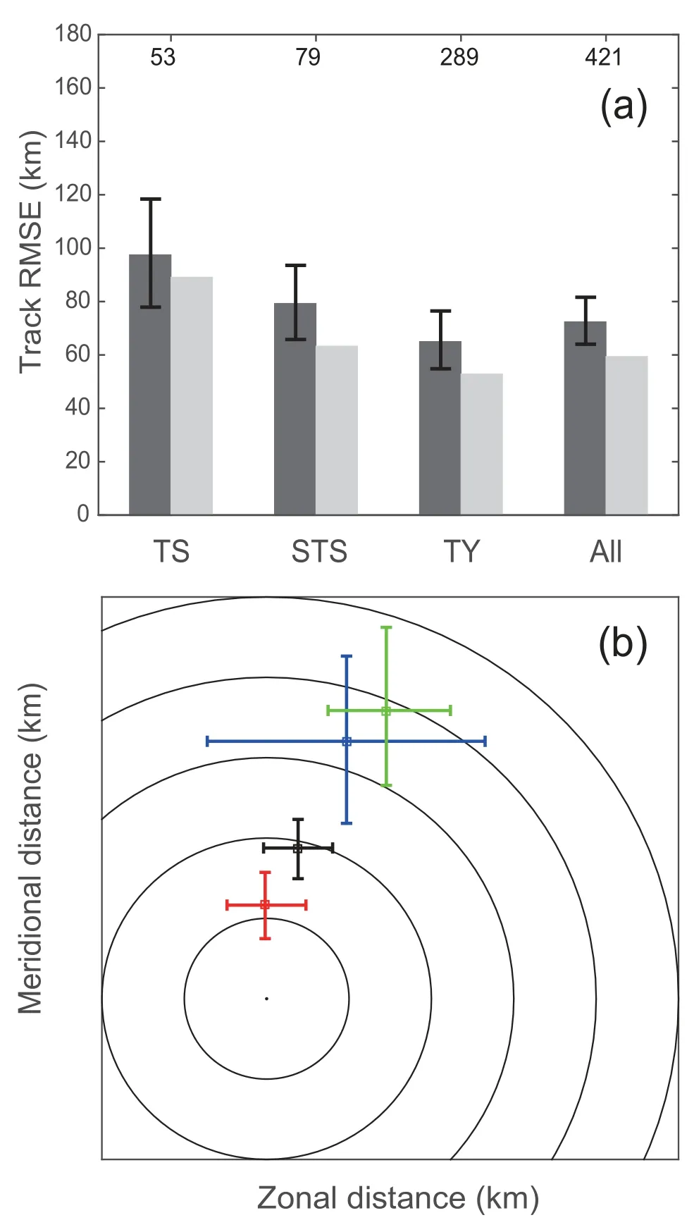
Fig. 2. (a) 6-h forecast ensemble mean RMS error (dark gray bar) and ensemble spread (light gray bar) of TC positions as a function of TC intensity. The number of verification times is given along the top. (b) 6-h forecast ensemble mean bias of TC positions for tropical storm (TS, blue line), severe tropical storm (STS, green line), typhoon (TY, red line), and all storms(ALL, black line). The range rings denote 10-km intervals.Error bars denote the 5% and 95% percentiles determined from bootstrap resampling.

Fig. 3. (a) 6-h forecast ensemble mean RMS error (dark gray bar) and ensemble spread(light gray bar) of TC minimum SLP as a function of TC intensity. The number of verification times is given along the top. (b) 6-h forecast ensemble mean bias of TC minimum SLP as a function of TC intensity. (c) As in (a), but for the TC maximum wind speed. (d) As in (b), but for the TC maximum wind speed. Error bars denote the 5% and 95% percentiles determined from bootstrap resampling.

Fig. 4. RMS error of TC positions for 5-d forecast as a function of forecast hour for (a) TS, (b) STS, (c) TY,and (d) ALL. The blue solid line denotes the WRF/EnKF forecast launched from ensemble mean analysis,and the red and black solid lines are the NCEP GFS forecast and ECMWF forecast, respectively. The number of verification times for WRF/EnKF and NCEP is given by the first row along the top, and the number of verification times for ECMWF is given by the second row along the top. Error bars denote the 5% and 95%percentiles determined from bootstrap resampling.

The lifetime durations and categories of the 21 TCs are given in Table 1. The lifetime durations of the storms ranged from 24 h (Rai) to 11 days (Lionrock). There were short-lived storms, such as Rai, Nida, Lupit, and Aere, and long-lived storms, such as Sarika, Chaba, Malakas, and Lionrock. According to the Regional Specialized Meteorological Centre (RSMC) Tokyo’s tropical cyclone intensity scale(Typhoon Committee, 2015), there were five tropical storms(TS) (Lupit, Conson, Dianmu, Kompasu, and Rai), whose maximum wind speeds were less than 24.2 m s-1; and there were five severe tropical storms (STS) (Mirinae, Nida,Omais, Chanthu, and Aere), whose maximum wind speeds were less than 32.4 m s-1. The remaining storms reached typhoon (TY) scale, with maximum wind speeds larger than 32.4 m s-1. Based on the Kaplan-DeMaria criteria (Kaplan and DeMaria, 2003), all the typhoons were characterized by at least one instance of rapid intensification (maximum wind speed increasing more than 15.4 m s-1per 24 h). Both Malakas and Songda met the rapid intensification criteria twice during their lifetimes. A wide variety of TC intensities are captured in this study.

4.Cycling verification

In this section, the cycling WRF/EnKF system is evaluated. Ensemble priors, i.e., 6-h ensemble forecasts, are verified against the JTWC advisory TC track position and intensity estimates that are the same as the assimilated quantities.The simulated TC position is given by the location of the minimum SLP. Figure 2 shows the TC track RMS errors, ensemble spread, and biases (observation minus forecast) for tropical storms (TS), severe tropical storms (STS), typhoons(TY), and all TCs (ALL), respectively. Figure 3 represents the RMS errors and biases of TC minimum SLP and maximum wind speed for different TC categories. The statistical significances of RMS errors and biases are determined using a bootstrap resampling with replacement method(Efron and Tibshirani, 1993). Each error distribution is resampled 1000 times with a bootstrap process. Error bars denote 5% and 95% percentiles; thus, only significance levels greater than 90% are considered statistically significant.

For all TC categories, the ensemble spread of TC position is slightly smaller than the RMS error. As shown by Anderson(1996) and Hamill (2001), verification of an ensemble forecast can be affected by the used imperfect observations. The ensemble spread here does not take into account the observation uncertainties; thus, the generally consistent TC position error with ensemble spread indicates a well calibrated ensemble being provided by the WRF/EnKF system (Houtekamer et al., 2005). The TC position error and spread of ALL are dominated by those of TY, because TY has many more samples than TS and STS. The position error and spread are inversely proportional to the TC intensity. This may be a result of poorly defined TC centers for weak TCs. Note that the 6-h track errors are larger than the operational forecast errors because there are ensemble members with large track errors, especially when the vortex is weak (figures are not shown). The zonal and meridional position biases of TY are also much smaller than those of TS and STS. For all instances, there are larger meridional position biases than zonal position biases, which is consistent with the persistently positivev-wind biases (figures are not shown).

Unlike for TC position, the ensemble spread of minimum SLP is insufficient to present the ensemble mean error, especially for TY. Similarly, the magnitude of TC maximum wind speed suffers from a large mismatch between the ensemble mean error and ensemble spread. Thus, the ensemble spread is not calibrated well for TC minimum SLP and maximum wind speed. TY has a much larger minimum SLP error than TS and STS, but the ensemble spread does not increase much from TS/STS to TY. Compared to TS and STS, the larger minimum SLP error of TY is also accompanied by a larger bias. TS and STS have similar errors of approximately 7 hPa, and similar biases of approximately +/- 0.75 hPa; but TY has an increased error of 22.21 hPa and an increased bias of -13.12 hPa. Although TS has a similar minimum SLP error and absolute bias to STS, TS has a larger maximum wind speed error and bias than STS. The error (bias) of maximum wind speed is 12.59 m s-1(-9.06 m s-1) for TS, 7.37 m s-1(-3.24 m s-1) for STS, and 14.61 m s-1(9.5 m s-1) for TY. Therefore, given a 6-km horizontal grid spacing, the WRF model is still unable to resolve the large gradients of TY’s wind and mass fields.The WRF/EnKF system overestimates the maximum wind speed for weak storms like TS and STS, but underestimates the minimum SLP and maximum wind speed for strong storms like TY.

5.Forecast verification

In this section, WRF/EnKF TC track and intensity deterministic forecasts launched from the ensemble mean analyses every 6 h are evaluated against the JTWC advisory TC track position and intensity estimates. For comparison, errors of the NCEP Global Ensemble Forecast System (GEFS) forecast(Zhou et al., 2017) and European Centre for Medium-Range Weather Forecasts (ECMWF) Ensemble Prediction System(EPS) global forecast (details are available online at https://www.ecmwf.int/sites/default/files/elibrary/2012/14557-ecmwf-ensemble-prediction-system.pdf) are also computed at the equivalent time. The NCEP GEFS has one control member and 20 ensemble members, and the 21 total ensemble members are integrated with the GFS model at approximately 34-km horizontal grid spacing for the first 8-d forecasts.The ECMWF EPS contains one control member and 50 ensemble members, and the 51 total ensemble members have a grid spacing of about 32 km through the 10-d forecast. Since WRF/EnKF uses a single forecast from the ensemble mean analysis, deterministic forecasts from the control members of the NCEP GEFS and ECMWF EPS are used for comparison in this section. Please note that WRF/EnKF has much higher horizontal grid resolutions (18 km, 6 km,and 2 km) than NCEP and ECMWF for the vortexes.

Instead of launching a deterministic forecast from the ensemble mean analysis, Torn (2010) and Cavallo et al.(2013) used a single member of the WRF/EnKF analysis ensemble for the deterministic forecast in order to avoid the overly smoothed depiction of the TC mass and wind fields which result from ensemble averaging. The single-member initial condition is chosen as the closest member to the ensemble mean analysis based on normalized latitude, longitude,and minimum SLP differences. To show the differences of a single forecast from the ensemble mean analysis or from a single ensemble member, a 5-d deterministic forecast is run from the ensemble mean analysis and a randomly chosen ensemble member every 6 h for 5 TS, 5 STS, and 8 TY.Results show that the deterministic forecast from the ensemble mean analysis and that from a single ensemble member have similar errors of minimum SLP and maximum wind speed through the 5-d forecast period (figures are not shown). The forecast from the ensemble mean analysis has track RMS errors similar to those from a single ensemble member within 48 h, and the former has smaller track RMS errors than the latter beyond 48 h, although the differences are not statistically significant at a 90% confidence interval.Therefore, the deterministic forecast from the WRF/EnKF ensemble mean analysis is used here and compared to the control forecast of NCEP GEFS and ECMWF EPS.

Figure 4 shows the track RMS errors as a function of forecast hours for TS, STS, TY, and ALL, respectively. The statistical significance of RMS error is denoted by the error bars showing 5% and 95% percentiles. The number of verification times is denoted on the top of the figure. The sample sizes of WRF/EnKF and NCEP are larger than that of ECMWF because WRF/EnKF and NCEP GEFS forecasts are computed every 6 h while the ECMWF EPS forecast is computed every 12 h. For TS, STS, TY, and ALL, WRF/EnKF deterministic forecasts generally have significantly larger track RMS errors than NCEP and ECMWF forecasts at short forecast lead times. The large initial track errors of WRF/EnKF are mainly resulted from the ensemble mean initial conditions, which have degraded initial position due to the ensemble averaging and have a subsequently fast error growth rate for the first 6 h due to imbalanced mass and wind fields of the ensemble mean. WRF/EnKF has insignificantly larger track errors or significantly smaller track errors than NCEP and ECMWF at long forecast lead times. Moreover, the meridional and zonal track biases of WRF/EnKF,NCEP, and ECMWF generally increase with forecast lead times, while the meridional track biases are larger than the according zonal track biases, especially at longer forecast lead times for TS and STS (Fig. 5). The meridional and zonal position error differences at longer forecast lead times are consistent with those from 6-h priors, which is possibly due to the persistently positivev-wind biases. Consistent with track RMS errors, WRF/EnKF deterministic forecasts in general have smaller track biases than NCEP and ECMWF at long forecast lead times. Thus, the regional simulation cannot better represent the large-scale environment compared to the global simulation, especially at short forecast lead times.

Fig. 5. Biases of TC positions from 5-d forecasts for (a) TS, (b) STS, and (c) TY. The blue dot, green plus,and red square denote WRF/EnKF forecasts launched from the ensemble mean analyses, NCEP GEFS control forecasts, and ECMWF EPS control forecasts, respectively. The range rings denote 200-km intervals.

Fig. 6. Same as Fig. 4, except for RMS error of TC minimum SLP.

Fig. 7. Same as Fig. 4, except for bias of TC minimum SLP.

Figures 6 and 7 display RMS errors and biases of minimum SLP as a function of forecast hour for different categories, respectively. For TS, WRF/EnKF deterministic forecasts produce larger RMS errors of minimum SLP than NCEP and ECMWF until about 60 h, and the error differences between WRF/EnKF and NCEP/ECMWF are not statistically significant at long forecast lead times. WRF/EnKF and NCEP (ECMWF) forecasts have negative (positive) biases of minimum SLP at short forecast lead times, while WRF/EnKF and ECMWF (NCEP) forecasts have negative (positive) biases for forecast lead times longer than 48 h. For STS, NCEP and ECMWF forecasts obtain similar RMS errors of minimum SLP, which are smaller than those of WRF/EnKF. Consistently, NCEP and ECMWF forecasts have similar biases of minimum SLP, which have smaller magnitudes than the positive biases of WRF/EnKF. For TY,WRF/EnKF deterministic forecasts generally have significantly smaller RMS errors of minimum SLP than NCEP and ECMWF until forecast lead times of 42 h and 72 h,respectively. Consistent with the RMS errors, NCEP and ECMWF forecasts have similar negative biases of minimum SLP, which have much larger magnitudes than the biases of WRF/EnKF. The RMS errors and biases of minimum SLP for ALL are similar to those of TY since the samples from TY are larger than those from TS and STS and thus the features of TY dominate.

The RMS errors and biases of maximum wind speed at 10 m as a function of forecast hour for different categories are shown in Figs. 8 and 9, respectively. For TS, WRF/EnKF deterministic forecasts have similar RMS errors of maximum wind speed to NCEP and ECMWF within 36 h but larger RMS errors than NCEP and ECMWF beyond 48 h.Similar biases of maximum wind speed are obtained for WRF/EnKF, NCEP, and ECMWF forecasts. For STS, WRF/EnKF deterministic forecasts have larger RMS errors of maximum wind speed than NCEP and ECMWF. Meanwhile,WRF/EnKF deterministic forecasts have negative biases of maximum wind speed, and the magnitudes are larger than those from NCEP and ECMWF. Different from the weak storms, WRF/EnKF deterministic forecasts produce significantly smaller RMS errors of maximum wind speed than NCEP and ECMWF for TY. The error differences among WRF/EnKF, NCEP, and ECMWF beyond 90 h are generally not statistically significant. Consistently, WRF/EnKF deterministic forecasts produce positive biases of maximum wind speed, and the magnitudes are much less than those of NCEP and ECMWF. Similar results to the comparisons for TY are obtained for ALL.

Therefore, although WRF/EnKF deterministic forecasts generally have larger RMS errors of minimum SLP and maximum wind speed than NCEP and ECMWF for weak storms like TS and STS, WRF/EnKF deterministic forecasts produce smaller RMS errors of intensity than NCEP and ECMWF for strong storms like TY. For weak storms, WRF/EnKF deterministic forecasts often have positive biases of minimum SLP and negative biases of maximum wind speed, which indicates overestimation of the intensity. For strong storms,WRF/EnKF deterministic forecasts often have negative biases of minimum SLP and positive biases of maximum wind speed, which indicates underestimation of the intensity. The underestimation of TY intensity is much better mitigated for WRF/EnKF compared to NCEP and ECMWF.There are environmental factors that may have influences on the vortex intensity, including temperature, specific humidity, vertical wind shear, etc. Figure 10 shows the profiles of differences for the mean specific humidity between WRF/EnKF and ECMWF forecasts. For each forecast, the mean specific humidity is averaged over an annulus that is centered around each vortex location with outer and inner circle radii of 5° and 2°, respectively. For weak storms, WRF/EnKF produces larger values of specific humidity below 500 hPa than ECMWF, which contributes to the intensity overestimation of weak vortexes for the WRF/EnKF. For strong storms,WRF/EnKF also has moister conditions than ECMWF,which explains the much better mitigated underestimation of TY intensity of WRF/EnKF compared to ECMWF.

6.Ensemble forecast performance

Performances of the ensemble forecasts for the typhoons listed in Table 2 are evaluated in this section. The mean absolute errors of the ensemble-mean position and intensity forecasts are compared with the mean ensemble spread.The consistency between these two quantities indicates that the ensemble contains an appropriate amount of variance,while the inconsistency between these two quantities indicates a lack of growing modes or reflecting model biases.For comparison, the mean absolute errors and ensemble spreads of NCEP GEFS and ECMWF EPS forecasts are also computed, as shown in Fig. 11.

Fig. 8. Same as Fig. 4, except for RMS error of TC maximum wind speed.

Fig. 10. Profiles of the differences of the mean specific humidity between WRF/EnKF and ECMWF 48-h forecasts for (a) STS and (b) TY. For each forecast, the mean specific humidity is the averaged specific humidity over an outer circle centered around each vortex with a 5° radius minus that over an inner circle with a 2° radius.

Fig. 11. The mean absolute error (solid) and ensemble spread(dashed) from ensemble forecasts of typhoons listed in Table 2 as a function of forecast hour for (a) track, (b) minimum SLP,and (c) maximum wind speed. The blue lines denote the WRF/EnKF forecast, and the red and black lines displays the NCEP GEFS and ECMWF EPS forecasts, respectively.

Fig. 12. 5-d ensemble forecast (a) tracks, (b) minimum SLP,and (c) maximum wind speed for typhoon Meranti from 0000 UTC 10 September. The thin blue, red, and green lines show the forecast values of the WRF/EnKF, NCEP, and ECMWF ensemble forecasts, respectively; and the thick lines denote the according ensemble mean. The black line denotes the observed value.

Fig. 13. Same as Fig. 12, except for typhoon Sarika from 1200 UTC 12 October.

For TC track, the mean absolute errors and ensemble spreads of WRF/EnKF, NCEP, and ECMWF ensemble forecasts are comparable within 30 h. Beyond that, the mean absolute errors of WRF/EnKF and NCEP, especially NCEP,increase at a higher rate than the ensemble spread; but the ensemble track forecasts of ECMWF have an even larger ensemble spread than the error. Thus, the ensemble track forecasts of WRF/EnKF and NCEP are underdispersive, while the ensemble track forecasts of ECMWF are overdispersive.For minimum SLP and maximum wind speed, WRF/EnKF,NCEP, and ECMWF ensemble forecasts contain appropriate variance when the forecast hour is less than 18 h. Beyond that, all three ensemble forecasts have spread deficiency.Compared to the ensemble forecasts of NCEP and ECMWF,WRF/EnKF ensemble forecasts have smaller intensity errors but contain larger ensemble spread. Therefore, WRF/EnKF ensemble forecasts lack variance for TC track (Puri et al., 2001; Magnusson et al., 2008; Torn, 2010), but WRF/EnKF provides better intensity ensemble forecasts than NCEP and ECMWF. Numerous factors have impacts on the ensemble forecasts, like the ensemble initial conditions,numerical model and parameterization schemes for different physical processes, model error representations, etc. A systematic investigation for the ensemble forecasts of different ensemble systems will be reported in a future study.

To illustrate the ensemble performance in detail, ensemble forecasts for typhoon Meranti from 0000 UTC 10 September and typhoon Sarika from 1200 UTC 12 October by the WRF/EnKF, NCEP, and ECMWF are shown in Figs. 12 and 13, respectively. The track ensemble forecasts for typhoon Meranti by WRF/EnKF, NCEP, and ECMWF all have the ensemble plumes centered on the observed value;thus, typhoon Meranti appears predictable. The ensemble forecasts of the minimum SLP and maximum wind speed by the NCEP and ECMWF show some degree of confidence, but they are far from the observed intensity. The intensity ensemble forecasts by WRF/EnKF are much closer to the observed values than the ensemble forecasts by NCEP and ECMWF; WRF/EnKF predicts a central pressure that is approximately 40 hPa lower than NCEP and ECMWF and a wind speed that is about 20 m s-1stronger than NCEP and ECMWF. Typhoon Sarika also appears predictable from the track ensemble forecasts, although WRF/EnKF shows less predictability than NCEP and ECMWF. Similar to typhoon Meranti, the intensity ensemble forecasts for typhoon Sarika by NCEP and ECMWF are far from the observed value, and all ensemble members fail to capture the re-intensification process. However, the intensity ensemble forecasts by WRF/EnKF have the ensemble plume around the observed intensity, and most ensemble members predict the re-intensification process. At forecast lead times from 12 h to 120 h,WRF/EnKF ensemble members for typhoons Meranti and Sarika have moister conditions than ECMWF at low levels(figures are not shown), which could explain the stronger vortexes predicted by WRF/EnKF. Therefore, consistent with previous error statistics based on the mean absolute error and ensemble spread, WRF/EnKF has better intensity predictability than NCEP and ECMWF.

7.Conclusions

This study describes the performance of a cycling WRF/EnKF system during most of the 2016 WNP typhoon season. Conventional in situ data, radiance observations, and TC minimum SLP are assimilated every 6 h using an 80-member ensemble. For the 21 storms during the experimental period, a 5-d deterministic forecast is launched from the ensemble mean analysis every 6 h within the duration of each storm; and a 5-d ensemble forecast is produced from the ensemble analyses for 7 typhoons whose intensities are underestimated. The forecast errors are compared to the ECMWF and NCEP operational models.

For all TC categories, the 6-h ensemble prior estimates of TC position from the WRF/EnKF system contain an appropriate amount of variance, while the TC intensity estimates are variance-deficient for all intensities, especially for TY.The TC position RMS error and spread are inversely proportional to the TC intensity, which may be a result of poorly defined TC centers for weak TCs. All TC instances are characterized by larger meridional position bias than zonal position bias. Category TY has much larger minimum SLP errors and biases than categories TS and STS, which indicates that a 6-km horizontal grid spacing is still unable to resolve the large gradients of TC wind and mass fields. Maximum wind speed errors and biases indicate that the WRF/EnKF system tends to overestimate maximum wind speed for TS and STS,but underestimate maximum wind speed for TY.

Compared to the NCEP and ECMWF operational control forecasts, the WRF/EnKF deterministic forecasts from the ensemble mean analyses often has larger TC track errors for all categories because the regional simulation cannot better represent the large-scale environment compared to the global simulation. A blending method that merges the analyses of global and regional models can be beneficial for TC track forecasting (Hsiao et al., 2015). The meridional track biases of WRF/EnKF, NCEP, and ECMWF are generally larger than the according zonal track biases for TS and STS,while WRF/EnKF and ECMWF produce much smaller zonal and meridional track biases than NCEP for TY. The WRF/EnKF deterministic forecasts exhibit smaller TC intensity errors for TY than the NCEP and ECMWF control forecasts, which is due to the higher grid resolution of the WRF/EnKF system; but the WRF/EnKF forecasts have larger TC intensity errors for TS and STS. The WRF/EnKF deterministic forecasts often have positive biases of minimum SLP and positive biases of maximum wind speed for weak storms, which means overestimation of the intensity. The NCEP and ECMWF control forecasts have negative biases of minimum SLP and positive biases of maximum wind speed for strong storms, which means underestimation of the intensity, but the WRF/EnKF deterministic forecasts produce smaller intensity biases than the NCEP and ECMWF control forecasts. Profiles of specific humidity differences between WRF/EnKF and ECMWF show that WRF/EnKF produces moister conditions than ECMWF for both weak and strong storms, which explains how WRF/EnKF overestimates intensity for weak storms and why WRF/EnKF has better mitigated underestimation of intensity for strong storms.

The ensemble forecasts from the WRF/EnKF system contain appropriate variance for TC track and intensity with short forecast lead times. With long forecast lead times, the ensemble forecasts of WRF/EnKF and NCEP are underdispersive for TC track, while the ensemble forecasts of ECMWF are overdispersive for TC track. The WRF/EnKF ensemble forecasts have smaller intensity errors but larger ensemble spread than the NCEP and ECMWF ensemble forecasts;thus, the WRF/EnKF system provides better TC intensity ensemble forecasts than NCEP and ECMWF, in terms of the comparison between amount of ensemble spread and mean absolute error. Moreover, the ensemble forecasts of WRF/EnKF can better capture the detailed intensity evolution than those of NCEP and ECMWF; thus, WRF/EnKF shows better intensity predictability than NCEP and ECMWF.

The large initial track errors of WRF/EnKF are possibly a result of fast error growth due to imbalances caused by data assimilation, which could be mitigated by appropriate initialization methods and will be reported in a separate study.To improve the WRF/EnKF ensemble forecasts with enlarged ensemble spread, advanced data assimilation that updates ensemble perturbations with hybrid background error covariance (Lei et al., 2021) and additive inflation that can represent model uncertainties (Whitaker and Hamill,2012) need be further studied. Moreover, the cycling ensembles and 5-d ensemble forecasts here provide a unique dataset for studying TC structure, dynamics, genesis, and predictability. Ensemble sensitivity analysis (e.g., Torn and Hakim, 2008; Lei and Hacker, 2015) using this output to understand the dynamical processes that limit the predictability of TC track, intensity, and structure will be presented in a future study. Data assimilation algorithms that can capture multiscale features of TCs and improve TC predictability will also be investigated.

Acknowledgements. We thank the editor and three anonymous reviewers for their insightful and constructive comments and suggestions. This work is jointly sponsored by the National Key R&D Program of China through Grant No. 2017YFC1501603, and the National Natural Science Foundation of China through Grant Nos. 41675052 and 41775057.

Open AccessThis article is licensed under a Creative Commons Attribution 4.0 International License, which permits use, sharing, adaptation, distribution and reproduction in any medium or format, as long as you give appropriate credit to the original author(s) and the source, provide a link to the Creative Commons licence, and indicate if changes were made. The images or other third party material in this article are included in the article’s Creative Commons licence, unless indicated otherwise in a credit line to the material. If material is not included in the article’s Creative Commons licence and your intended use is not permitted by statutory regulation or exceeds the permitted use, you will need to obtain permission directly from the copyright holder. To view a copy of this licence, visit http://creativecommons.org/licenses/by/4.0/.