Fang Zhou(周方) Chang Su(苏畅) Shuqi Xu(徐舒琪) and Linyuan L¨u(吕琳媛)

1Yangtze Delta Region Institute(Huzhou)&Institute of Fundamental and Frontier Sciences,University of Electronic Science and Technology of China,Huzhou 313001,China

2Beijing Computational Science Research Center,Beijing 100193,China

Keywords: social networks,fast influencers,final influencers,spreading dynamics,degree assortativity

1. Introduction

In network science, vital nodes identification[1–5]is an intriguing and important problem, which has attracted longstanding scientific attention. Vital nodes are considered as nodes that play an important role in the structure or function of networks. In the scenario of information spreading,[3,6]vital nodes are also known as influencers (or “influentials”),namely, those who can influence a large fraction of nodes in the spreading dynamics. Identifying influencers have crucial meanings on controlling or speeding the spreading process in networks and can support various practical applications. For example, in advertisement marketing campaigns,[1]having a celebrity promote a product on social media can largely enhance the visibility of the product, thus driving the product sales and obtaining a good marketing effect.

Researchers have made great efforts in the identification of influencers and have gained a series of achievements.[1–4,7–10]To determine whether a node in a network is an influencer, most research relies on quantifying the spreading capacity of the node in spreading dynamics.The spreading process is usually specified as follows: for a given network, we choose a node (typically referred to as the “seed node”) and employ a spreading model to simulate the spreading process; when the spreading stops, we measure the seed node’s spreading capacity, and the nodes with outstanding capacity are defined as influencers. Researchers have evaluated many methods’ ability to reproduce the ranking of nodes’ spreading capacity. One of the most effective and simplest methods is the centrality metric that considers the network structure of the focal node. Commonly-used centrality metrics that are introduced to rank nodes include local metrics such as degree,[11]H-index,[12]LocalRank,[3]collective influence,[4]and global metrics such as eigenvector centrality,[13,14]betweenness centrality,[15]closeness centrality,[16]dynamics-sensitive centrality,[17]etc. Besides,other iterative-based methods proposed by researchers include PageRank[18]and its parameter-free variant LeaderRank,[19]HITS,[20]and SALSA.[21]

Based on the above process of influencer identification,researchers mainly focus on the final spreading capacity of nodes (i.e., the result when the spreading is finished), but ignore nodes with great spreading capacity at the early stage.Zhouet al.[7]provided the first step towards uncovering this type of nodes, which they called “fast influencers”. The authors revealed that fast influencers are different from traditional influencers that pursue the final big impact, and they proposed a metric called social capital to identify them. Fast influencers are of both theoretical and practical significance.Potential applications include, for example, maximizing a newly-released movie’s promotion effect in a limited time and cutting off the spreading of the latest rumor as soon as possible.

Despite the fact that fast influencers and final influencers have a clear distinction on definitions, there lacks an understanding of the underlying differences between fast and final influencers,which is what we aim to achieve in this work. To this end, we focus on comparing the two types of influencers based on two network-based features: local structure[22]and degree assortativity,[23–25]which have been revealed to influence the spreading process in networks. Specifically, we analyze the differences between the fast and final influencers in terms of their spreading capacity and four local centrality metrics, degree,h-index,k-core and LocalRank, as well as study how the network degree assortativity influences the fraction of the two types of vital nodes.The structure of the paper is organized as follows,firstly in Section 2,we introduce the related approaches,definitions of fast-only and final-only influencers,and the details of eight studied datasets. Then in Section 3,we analyze the distinct spreading performance and local structures of fast-only influencers and final-only influencers, and discuss the relationship between the network degree assortativity and the fraction of fast-only/final-only influencers. In Section 4, we conclude the main results of this work and reveal insights for practical applications.

2. Method

2.1. Susceptible–infected–recovered model

We employ the susceptible–infected–recovered (SIR)model to simulate the spreading dynamics in networks. In the SIR model,there are three types of individuals:susceptible individuals,infected individuals,and recovered individuals,and there are two model parameters, infect probabilityβand recover probabilityμ. The SIR model supposes that infected nodes infect their neighboring susceptible nodes with probabilityβ, infected individuals recover to the recovered state with probabilityμ, and recovered individuals cannot be infected again. When a seed node is given,we assume that it is infected, and all other nodes are in the susceptible state, then the spreading proceeds according to the above rules. When no individual is found in the infected state,the spreading process ends, and the total number of nodes in the recovered state is measured as the spreading capacity(also referred to as spreading size or spreading effect)of the seed node.

2.2. Definition of the fast-only and final-only influencers

Fast influencers are considered as individuals that can influence the top fraction of individuals at the early stage of the spreading process.[7]In comparison,final influencers are those individuals whose spreading capacity is ranked among the top(according to a top ratiox%) at the final stage. In this paper, we focus on the non-overlapping parts between fast influencers and final influencers, which we refer to as fast-only and final-only influencers,respectively. Specifically,fast-only influencers are the fast influencers that do not belong to final influencers. Similarly,the final-only influencers are those final influencers that do not overlap with fast influencers. According to the definitions,fast-only influencers are individuals that achieve high spreading capacity at the early stage but lose the superiority at the final stage, and on the contrary, finalonly influencers are individuals that fail to exhibit a prominent spreading capacity at the early stage but influence a large fraction of nodes at the final stage. According to the same top ratio, the numbers of fast-only and final-only influencers are the same.

2.3. Assortativity coefficient

Assortativity coefficient(r)is the Pearson correlation coefficient of degrees between pairs of linked nodes.[26,27]A positiverdenotes that the high(low)-degree nodes tend to connect with high(low)-degree nodes,while a negativerindicates that the high(low)-degree nodes tend to connect with low(high)-degree nodes. In formula, the definition of the assortativity coefficient of a network is as follows:

wherewkis the distribution of the remaining degree(i.e., the probability that the neighboring node of a randomly-chosen node in the network has degreek) andejkis the joint probability distribution of the remaining degrees of the two nodes at either end of a randomly-chosen edge,andσ2wis the variance of the distributionwk,-1≤r ≤1. Whenr=1, the network is totally assortative(all nodes are only connected with nodes with the same degree)andr=-1 if the network is totally disassortative.

2.4. Degree configuration model

To reveal how degree assortativity influences the fraction of fast-only and final-only influencers in the network, we introduce the degree configuration model[28]into the analysis to adjust the degree assortativity of networks. Specifically,for a given network,the model keeps the degree sequence fixed and changes the assortativity of the network.[28–30]According to the degree configuration model,given a network,we randomly choose two edges,(v1,v2)and(v3,v4),which are guaranteed to be different. The four nodes are ranked with respect to their degrees.

To generate an assortative network from the original one,with probabilityp,we rewire the two edges to let one of them connects the two nodes with smaller degrees and the other link connects the two nodes with larger degrees; with probability 1-p, the two edges are randomly rewired. To avoid multiple edges connecting two same nodes, we will select a new pair of nodes if the rewired edge has already existed in the network. Such a process is repeated until the maximum iterations reaches. In this model,pcontrols the extent of degree assortativity. Ifpis close to 1,after the rewiring process,the generated network tends to be assortative. Similarly, through rewiring network edges with probabilitypto let nodes with larger degrees are connected with nodes with smaller degrees,we can generate networks with tunable disassortativity.

2.5. Centrality metrics

Centrality metrics measure the relative importance of a node in the network,which capture a node’s position features in the network structure.In the analysis,we focus on the structure of final-only influencers and fast-only influencers in terms of four metrics: degree,h-index,k-core, and LocalRank. We use aN×Nadjacency matrixAto represent the studied undirected un-weighted network,whereNis the number of nodes in the network,whereAi j=1 if there is a edge between nodeiandj,andAij=0 otherwise.

Degree Degree is the simplest centrality metric. In a network, nodei’s degreekiis defined as the number of its neighbors,[11]in formulaki=∑j Aij.

Theh-index Theh-index was firstly introduced to measure the academic impact of scholars[12]based on their publications and the corresponding citations. Then, it was extended to quantify nodes’ significance based on their neighbors’ impact.[31]For a given nodei, itsh-index is defined as the maximum valuehisuch thatihas at leasthineighbors whose degrees are all no less thanhi.

Thek-core The calculation of nodes’k-core is according to a network pruning process.[2]Specifically,the process starts by removing nodes with degrees equal to one, the pruning is continued until all nodes’degrees are larger than one,then thek-core of the removed nodes is one. Next,the pruning process is repeated for the remaining nodes with degreek=2,3,...,and all nodes will be assigned theirk-core scores.[2]

LocalRank For a given nodei, its LocalRank[3]scoreLRiis defined as

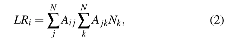
whereNkis the number of the nearest and the next nearest neighbors of nodek. LocalRank takes nodes’four-order local structure into account.

2.6. Empirical datasets

In the analysis, we use eight social network datasets to support our research. Email is a communication network at the University Rovira i Virgili in Tarragona in Spain,[22]nodes are users and each edge represents that at least one email between the corresponding two users was sent. Cond-mat is a collaboration network of scientists,[33]in which nodes represent scientists and each edge means the two linked scientists have co-authored at least one paper. Lastfm-asia is a social network of LastFM users,[34]nodes are LastFM users from Asian countries and edges are mutual following relationships between them. Musae-facebook is a page-page network of Facebook sites.[35]Nodes represent official Facebook pages (such as pages of politicians, governmental organizations, television shows and companies) and edges are mutual likes between sites. Deezer-HR, deezer-HU and deezer-RO are three friendship networks collected from the music streaming service Deezer from Croatia, Hungary, and Romania, respectively.[36]Nodes represent the users and edges are the mutual friendships. Facebook is a friendship network[37]in which nodes represent Facebook users,and edges represent the mutual friendships. We summarize the characteristics of the eight datasets in Table 1.

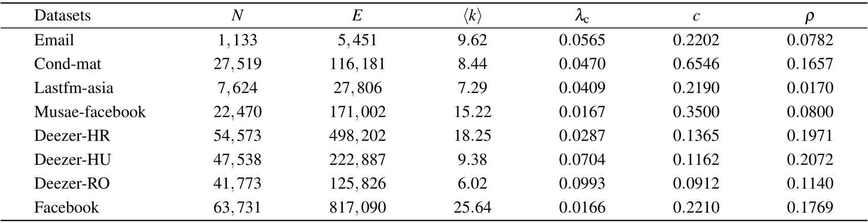
Table 1. The characteristics of the eight studied datasets. Here N is the size of network(i.e.,number of nodes),E is the number of edges,〈k〉is the average degree,λc is the threshold in the SIR model,[38] c is the clustering coefficient,and ρ is the degree assortativity.

3. Results

3.1. Overlap between fast influencers and final influencers

To identify the fast and final influencers and analyze the differences between them,we employ the SIR model[2,39](see Subsection 2.1 for details) to simulate the spreading dynamics. In the simulation,the recover probability holds for a fixed value ofμ=1, and the infect probabilityβchanges fromλcto 8λc. Given nodei, we set it as the seed infected node to start the spreading process and recordi’s spreading capacity(i.e.,number of infected individuals)at timetasqi(t). When the spreading process ends, we denotei’s final spreading capacity asqi. We implement 100 times simulation to obtain average results. After obtaining all nodes’spreading capacity at any given time,we rank all individuals’q(t)and define the topx%(x=1,2,5)as the fast influencers at timet=5. Similarly,ranking all individuals’q,and the topx%(x=1,2,5)of individuals are defined as final influencers.

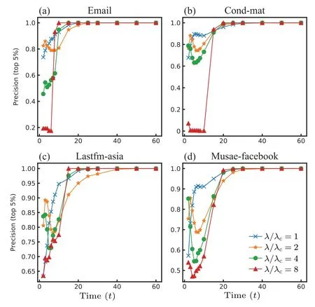
Fig. 1. The overlapping fraction between fast influencers and final influencers on four social networks.Different curves in each panel denote the results based on different λ/λc, where λc is the threshold value of SIR model.[2,39] The result shows that in the four networks, with the increase of t,the curves decrease at first,then increase.

Under different time steps (t), we calculate the overlapping fraction between the fast influencers(top 5%byq(t))and final influencers(top 5%byq),which is denoted as precision(top 5%). Precision represents the fraction of fast influencers that become the final influencers at the final stage. The results on four social networks (see Subsection 2.6 for details) are presented in Fig.1. We find that as the time(t)increases,the overlap between fast influencers and final influencers exhibits an overall decreased trend firstly and then increased trend.The results are consistent under the condition of other top ratios, see the results of top 1% and 2% in Figs. A1 and A2 in Appendix A.And the results on the other four datasets are shown in Figs. A3–A5, which indicates a monotonically increasing trend. The discrepancy could be due to the difference in network size, namely, compared with the four networks in Fig.1,and Deezer and Facebook are larger,in which the same top ratio involves more nodes, which could distort the initial trend of the curve. In all studied datasets,the precision value reaches 1 within 60 time steps,which indicates the spreading ends beforet=60. Consistent with the prior study about fast influencers,[7]we define nodes with the top 5%q(5) as fast influencers in the following analysis, which also corresponds to a low overlap between the two types of influencer.

Further,we analyze how the spreading parameterλ(λ=β/μ) influences the overlap between the fast influencers and the final influencers. As mentioned above, in the SIR model,we fix the recover probabilityμ=1, and change the infect probabilityβto obtain differentλ. Whenλis large thanλc(the threshold of the SIR model,[5,38]see Table 1), i.e.,λ/λc＞1, the spreading outbreaks; whenλis smaller thanλc(λ/λc＜1),the spreading will vanish soon. In our simulation,under different infect probabilities,for a given seed nodei,the spreading process is implemented 100 times to obtain average results. We plot the results under four differentλ/λcin Fig.1.The results demonstrate that whent=5,the overlap between the two types of influencers becomes smaller with a largerλ,revealing that in a scenario with high infected probability,one needs to carefully consider the specific type of influencers he wants to identify, because in this case, few final influencers would be fast influencers at the same time. The results are robust in terms of different top ratios and other four datasets(see Figs.A1–A5).

3.2. Fast-only influencers versus final-only influencers

Both fast-only influencers and final-only influencers are of importance to practical applications. For example, in advertisement marketing, the marketer sometimes is more concerned about maximizing the advertisement effect at the early stage, thus spending on the fast-only influencers is a better choice to balance the efficiency and cost. On the contrary, if the goal of the marketer is the long-term effect, focusing on final-only influencers is a better choice that will bring a longlasting marketing effect.Therefore,having a deep understanding of the difference between fast-only influencers and finalonly influencers is crucial for making rational use of them.

3.2.1. Comparison of spreading capacity

To measure the gap of spreading capacity between the fast-only influencers and the final-only influencers,we calculate the average spreading capacity of the two types of individuals at different time. The results on four datasets are shown in Fig.2(see Fig.A6 for the results of the other four datasets),in which each column denotes the results based on differentλ/λc. In the four datasets, we observed consistent patterns.Firstly, by their definitions, final-only influencers underperform fast-only influencers at the early stage, but they can exhibit high spreading capacity in the final stage. Secondly,fastonly influencers perform well at the early stage but lose their superiority at the late time. Thirdly,the average spreading capacity of fast-only influencers and final-only influencers is always better than that of the random-chosen(5%)individuals.

Fig.2. The spreading capacity of fast-only influencers,final-only influencers and random-chosen individuals. The x-axis is the time t,and the y-axis is the average spreading capacity of the three types of nodes. Different columns denote results based on different λ/λc.

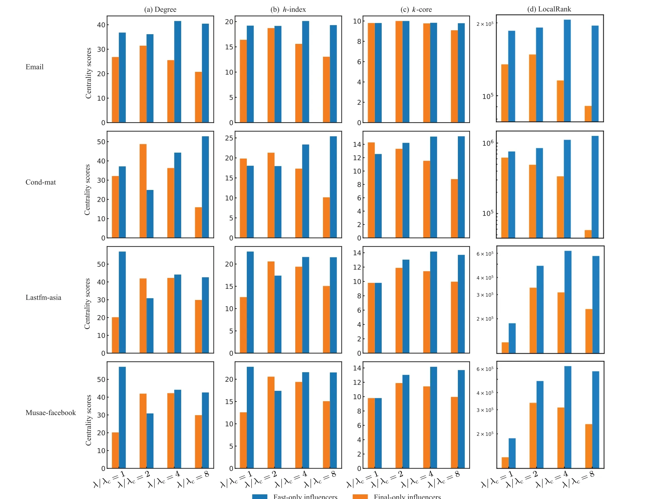
Fig.3.The average local metric scores of fast-only influencers and final-only influencers on the four social networks.The local metrics include degree,h-index,k-core and LocalRank. The x-axis denotes four different λ/λc, and the y-axis denotes the average centrality scores of two types of influencers. In general,the results indicate that compared with final-only influencers,fast-only influencers have more strong local structures,as λ/λc increases,the score gap between fast-only influencers and final-only influencers becomes wider.

Finally, the last intersection between the curves of finalonly influencers and fast-only influencers (the time that the spreading capacity of the former exceeds that of the latter)gradually moves backward as the increase ofλ, which indicates that under a condition of high spreading probability,final-only influencers need more time to exceed fast-only influencers.

3.2.2. Comparison of local structure via centrality metrics

Next, we compare the local structure of fast-only influencers and final-only influencers by computing their average centrality metric scores(see Subsection 2.5). Figure 3 shows the results of fast-only and final-only influencers. The metrics include degree,h-index,k-core and LocalRank(the results on the other four datasets are shown in Appendix Fig.A7). From Fig. 3, we find that compared with the final-only influencers,the fast-only influencers have higher scores with respect to all considered four metrics. Similar results are observed on the other four datasets, which reveal that nodes with strong local structures tend to have a powerful ability to infect more nodes at the early stage. The results indicate that to maximize the spreading effect in a limited time,we need to emphasize more on individuals’ local structure than global structure, which is consistent with the finding in previous work.[7]On the contrary, to achieve a long-time spreading effect, we should not only consider the local position of individuals, but also consider the global position of individuals.[5]

Figure 3 also demonstrates that asλincreases,the score gap between fast-only influencers and final-only influencers becomes larger,which is consistent with the results in Fig.1,namely, in the case of large infected probability, the discrepancy between fast-only influencers and final-only influencers becomes larger, non-top-spreading individuals at the early stage have more chance to become final influencers in the final stage.

3.3. The impact of degree assortativity on the fraction of fast-only/final-only influencers

Previous research has claimed that the degree assortativity of networks influences the spreading dynamics.[23–25]In this section,we investigate how the variation of degree assortativity influences the fast-only and final-only influencers. To this end, we adjust the degree assortativity of given networks by the configuration model,[28]which keeps the degree sequence fixed and changes the degree assortativity of networks by rewiring the edges(see Subsection 2.4 for details). To obtain robust results, for each dataset, we run the configuration model 10 times and analyze the average results.

Recall that in the configuration model, parameterpcontrols the extent of the network assortativity or disassortativity.In Figs. 4(a) and 4(b), we show the relationship betweenpand the assortativityron four studied networks. Whenr ＞0,the network is assortative, which indicates that nodes tend to be connected with nodes with similar degree values,otherwiser ＜0. Taking the result on email network as an example, in panel a, we can see that whenpincreases from 0 to 1, the assortativity of the network rises from-0.03 to 0.51,indicating that the network tends to be more assortative. Similarly,in panel b, withpincreases from 0 to 1, the assortativity of email network declines from-0.03 to-0.37, which means the network tends to be more disassortative.

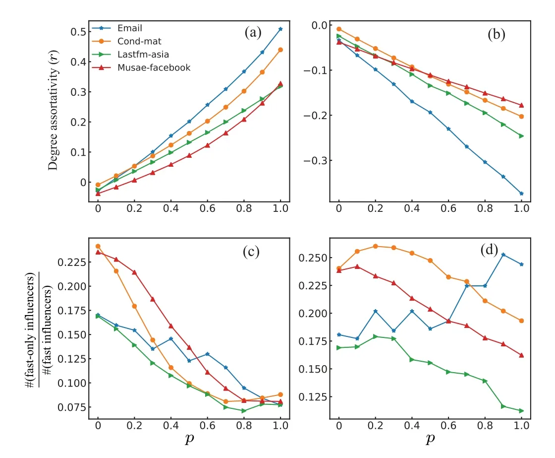
Fig.4. The influence of degree assortativity on the fraction of the fast-only and final-only influencers. In panels (a) and (b), the x-axis represents the parameter p in the configuration model,and the y-axis is the degree assortativity (r) of the network. In panel (a), with the increase of p, the curves go up, indicating that the generated networks become more assortative. Similarly, in panel (b), when p rises from 0 to 1, the curves go down, meaning that the generated networks become more disassortative. In panels (c) and(d),the y-axis denotes the ratio of the number of fast-only influencers to the number of fast influencers. In panel (c), when p increases, the fraction of fast-only influencers decreases on the four studied networks. In panel (d),when p increases, we do not observe a consistent pattern. Specifically, in cond-mat, lastfm-asia and muase-facebook, the increase of p is associated with the decrease of fast-only influencers,but in email network,the opposite is true.

We further study the relation between degree assortativity and the fraction of the fast-only and final-only influencers.For each generated network by the configuration model,[28]we run the SIR model and record all individuals’spreading capacity att=5 and at the end.Then we calculate the fraction of fast-only influencers. Figure 4(c)demonstrates that with the increase ofp,the fraction of fast-only influencers decreases. Such a result indicates that when a network becomes more assortative, fast influencers are more likely become final influencers, namely,ordinary individuals that did not perform well at the early stage can hardly achieve a top spreading effect at the final stage,and individuals in the network can hardly break the hierarchy in information spreading,which is unfair for most individuals.The reason for such a result is that if most nodes tend to connect with nodes with similar degrees,individuals with low degrees can hardly transmit information to high-degree nodes. As for Fig.4(d),it shows that when the network becomes more disassortative, the variation of the fraction of fast-only influencers is distinct on different datasets. In lastfm-asia, cond-mat and musae-facebook datasets,the fraction of fast-only influencers decreases as the networks become more disassortative,but for the email dataset, with the increase ofp, the fraction of fastonly influencers increases.

Following we discuss the possible reasons for this discrepancy. Based on the analysis of Fig. 4(b), we notice that compared with the other three networks, the email network is more disassortative withpincreases, indicating it involves a larger fraction of high-degree nodes that connect with lowdegree nodes for a givenp. And in our paper, the defined fast-only influencers are individuals with relatively high degree(see Fig.2 and Table 1 for details),which leads to the case that with the increase of degree disassortativity, comparing with other three networks,in email network,there have more high-degree nodes tend to connect with low-degree nodes,and the fractions of fast-only and final-only influencers increase as well. While for the other three networks, there are relatively fewer high-degree nodes that connect with low-degree nodes,the fraction of fast-only and final-only influencers would not increase. The results with respect to the other four datasets are shown in Appendix Fig. A8, which demonstrates that the deezer-HU and deezer-RO networks show similar results(the more disassortative the network is,the more chance that ordinary individuals have to become influencers finally).

In summary, our results indicate that for assortative networks,it is hard for those individuals that perform non-top at the early stage to achieve a breakthrough at the final stage,and individuals who perform well at the early stage have more chance to keep their superiority at the final stage.

4. Conclusion

Vital nodes play an important role in the structure and function of networks. In this paper, we distinguish two types of vital nodes: fast influencers and final influencers. We study the overlap between the two types of influencers at different time and spreading parameterλ. Then we focus on the non-overlapping parts of fast influencers and final influencers, which we call the fast-only influencers and final-only influencers, respectively, and we analyze the differences between them. We study howλinfluences the spreading capacity of the fast-only influencers and final-only influencers,and the result shows that increasingλwill make those individuals with non-top spreading performance have more chance to have top performance at the final stage. Then we compare the local structures of fast-only influencers and final-only influencers through centrality metrics, and find that on the studied eight social networks,compared with final-only influencers, the fast-only influencers have a stronger local structure, represented by higher centrality scores. Finally, we discuss how the degree assortativity influences the fraction of fast-only influencers. The result indicates that when the network becomes more assortative,individuals that perform well at the early stage will keep their superiority at the final stage.And mediocre individuals at the early time in the network can hardly achieve a high spreading effect at the final stage. Our research shows that if people focus on the effect at the early stage, they need pay more attention to fast-only influencers to reach a balance between effect and cost. If they are more concerned about the long-time effect, they need to focus on final-only influencers to achieve a long-lasting spreading effect. Our research can also shed the light on the sociology field, to keep the social system fairer, we need to make the society more disassortative rather than assortative.

Acknowledgements

L.L. acknowledges the Science Strength Promotion Programme of UESTC,Chengdu.

Project supported by the National Natural Science Foundation of China (Grant Nos. 61673150 and 11622538) and Special Project for the Central Guidance on Local Science and Technology Development of Sichuan Province,China(Project No.2021ZYD0029).

Appendix A: Overlap between fast influencers and final influencers for different top ratios and datasets

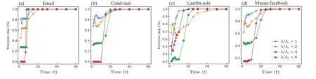
Fig.A1. The overlap between fast influencers and final influencers on four social networks(top 1%).

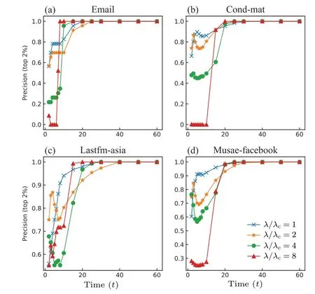
Fig.A2. The overlap between fast influencers and final influencers on four social networks(top 2%).

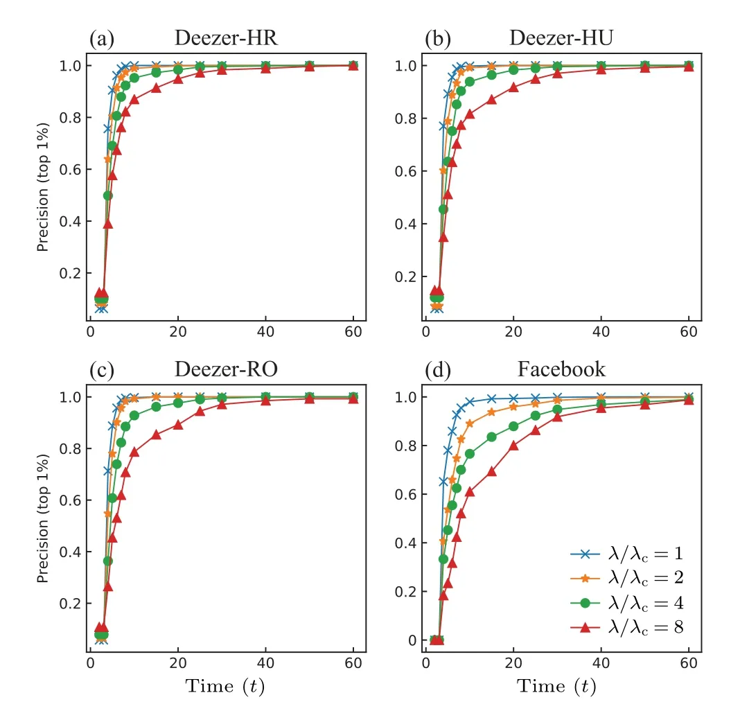
Fig.A3. The overlap between fast influencers and final influencers on deezer-HR,deezer-HU,deezer-RO,Facebook networks(top 1%).

Fig.A4. The overlap between fast influencers and final influencers on deezer-HR,deezer-HU,deezer-RO,Facebook networks(top 2%).

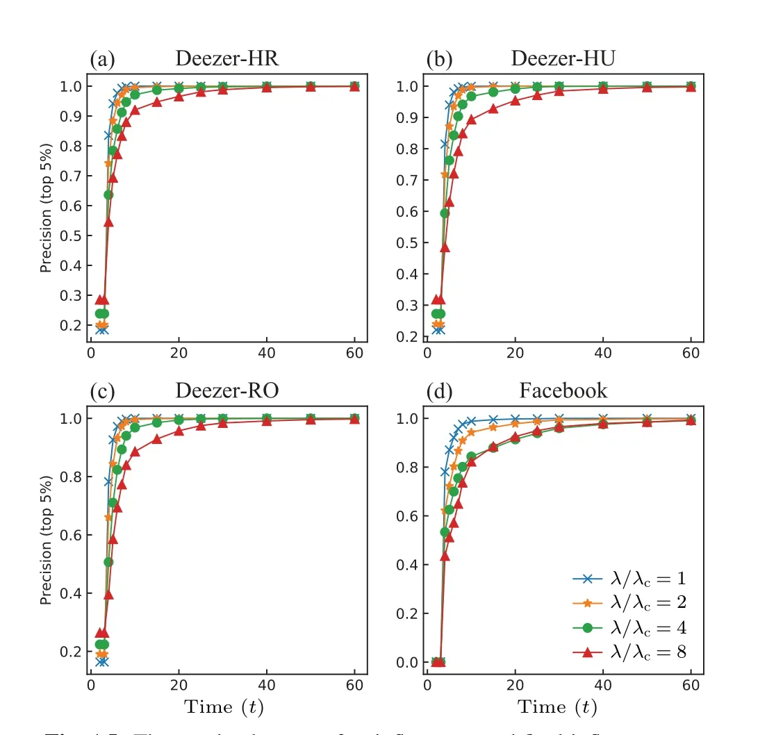
Fig.A5. The overlap between fast influencers and final influencers on deezer-HR,deezer-HU,deezer-RO,Facebook networks(top 5%).

Appendix B:The comparison between fast-only and final-only influencers in terms of spreading capacity at different time

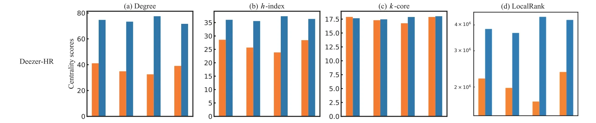
Fig.B1. The spreading capacity of the fast-only influencers,final-only influencers and random-chosen(5%)individuals on deezer-HR,deezer-HR, deezer-HR, Facebook networks. The x-axis is the time t, and the y-axis is the average spreading capacity of the three types of nodes.Different columns denote results based on different spreading parameters λ. Similar to Fig.3 in the main text,but for the other four datasets.

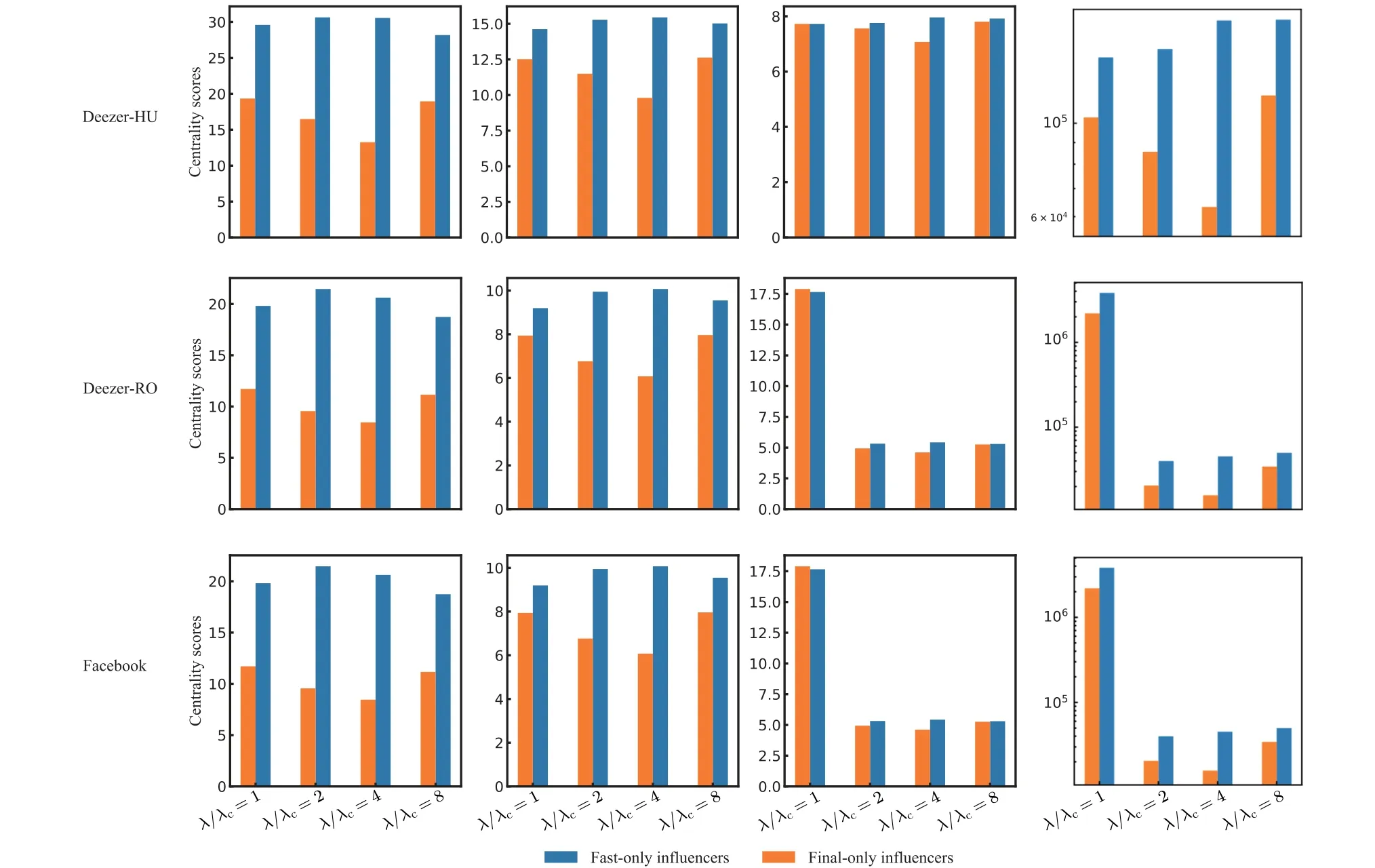
Fig.B1. The spreading capacity of the fast-only influencers,final-only influencers and random-chosen(5%)individuals on deezer-HR,deezer-HR,deezer-HR, Facebook networks. The x-axis is the time t, and the y-axis is the average spreading capacity of the three types of nodes. Different columns denote results based on different spreading parameters λ. Similar to Fig.3 in the main text,but for the other four datasets(continue).

Appendix C:Centrality metrics scores of fast-only and final-only influencers on four social networks

Fig.C1. The average local metric scores of the fast-only influencers and final-only influencers on the other four social networks. Similar to Fig.4 in the main text,but for the other four datasets.

Appendix D:The impact of degree assortativity on the fraction of fast/final-only influencers

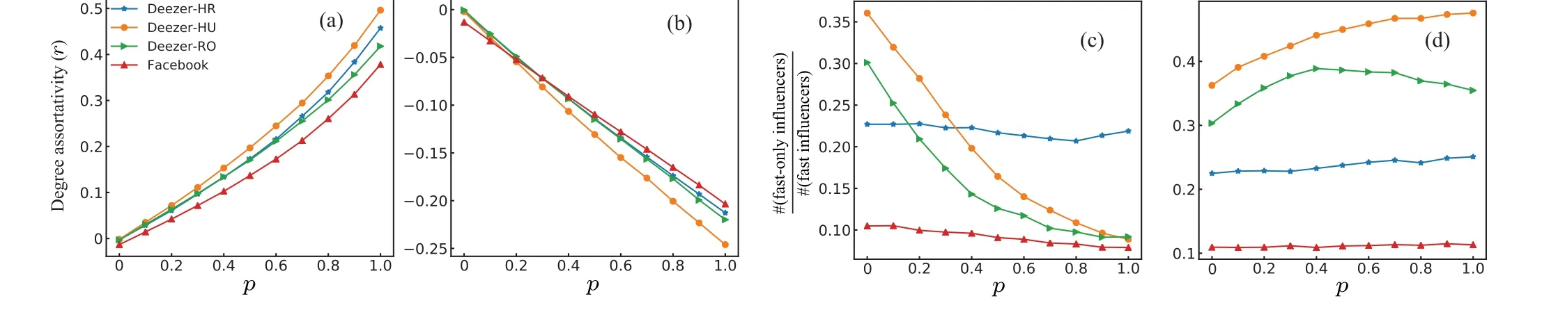
Fig.D1. The influence of degree assortativity on the fraction of the fast-only and final-only influencers. Similar to Fig.4 in the main text,but for the other four datasets.