Shi-Jie Pan(潘世杰) Lin-Chun Wan(万林春) Hai-Ling Liu(刘海玲) Yu-Sen Wu(吴宇森)Su-Juan Qin(秦素娟) Qiao-Yan Wen(温巧燕) and Fei Gao(高飞)

1State Key Laboratory of Networking and Switching Technology,Beijing University of Posts and Telecommunications,Beijing 100876,China

2State Key Laboratory of Cryptology,P.O.Box 5159,Beijing 100878,China

Keywords: quantum algorithm,quantum machine learning,amplitude amplification

1. Introduction

Quantum computing theoretically demonstrates its computational advantages in solving certain problems compared with classical computing, such as the problem of factoring integers,[1]unstructured data searching problem,[2]and matrix computation problems.[3–5]In recent years,quantum machine learning has received widespread attention as a method that successfully combines classical machine learning with quantum physics. An important direction of quantum machine learning is to design quantum algorithms to accelerate classical machine learning, including data classification,[6–9]linear regression,[10–14]association rules mining,[15]and anomaly detection.[16]

Dimensionality reduction (DR) is an important part of machine learning,which aims to reduce the dimensionality of the training data set while preserving the structure information of the data points as well as possible. The DR algorithm often serves as a preprocessing step in data mining and machine learning to reduce the time complexity of the algorithm and avoid a problem called “curse of dimensionality”.[17]Generally,The DR algorithms can be classified into two categories:the linear one and the nonlinear one. The most widely used linear DR algorithms include principal component analysis(PCA),[18]linear discriminant analysis(LDA),[19]and neighborhood preserving embedding (NPE),[20]while the typical nonlinear DR algorithm is locally linear embedding(LLE).[21]Here, we focus on NPE which can be regarded as the linear approximation of LLE. Unlike PCA that tries to preserve the global Euclidean structure, NPE aims at preserving the local manifold structure. Furthermore, NPE has a closed-form solution. Similar to other DR algorithms, NPE requires a large amount of computational resources in the big-data scenario because of its high complexity.

In recent years, some researchers successfully combined DR algorithms with quantum techniques and obtained various degrees of speedups. Lloydet al.[22]proposed a quantum PCA algorithm to reveal the large eigenvectors in quantum form of an unknown low-rank density matrix,which achieves an exponential speedup on the dimension of the training data.Latter, Yuet al.[23]proposed a quantum algorithm that compresses training data based on PCA, and achieves an exponential speedup on the dimension over the classical algorithm.Conget al.[8]proposed a quantum LDA algorithm for classification with exponential speedups on the scales of the training data over the classical algorithm. Besides,there are some other quantum DR algorithms, including quantum A-optimal projection,[24,25]quantum kernel PCA[26]and quantum spectral regression.[27,28]

For NPE,Lianget al.[29]proposed a variational quantum algorithm(VQA),called VQNPE,and expected to achieve an exponential speedup on dimensionalityn. NPE contains three steps,i.e., finding the nearest neighbors of each data point,constructing the weight matrix,and obtaining the transformation matrixA.VQNPE includes three quantum sub-algorithms with a VQA in the third sub-algorithm, corresponding to the three steps of NPE.However,VQNPE has two drawbacks: (i)The algorithm is incomplete. As the authors pointed out,it is not known how to obtain the input of the third sub-algorithm from the output of the second one. (ii) It lacks a provable quantum advantage.Since the advantage of VQA has not been proved rigorously yet(generally,we say that VQA has potential advantage[30,31]),it is hard to examine the speedups of the third sub-algorithm.

In this paper, we propose a complete quantum NPE algorithm with rigorous complexity analysis. Our quantum algorithm also consists of three quantum sub-algorithms, corresponding to the three steps of the classical NPE. The first one is finding the neighbors of each data point by quantum amplitude estimation and quantum amplitude amplification.By storing the information of neighbors in a data structure of QRAM,[32,33]we obtain two oracles. With these oracles, the second one reveals the classical information of the weight matrixWcolumn by column by quantum matrix inversion technique. In the third one,we use a quantum version of the spectral regression (SR) method to get the transformation matrixA. Specifically,we obtain thed(dis the dimension of the low dimensional space) bottom nonzero eigenvectors of the matrixM=(I-W)T(I-W) at first, and then perform several times of the quantum ridge regression algorithm to obtainA.As a conclusion,under certain conditions,our algorithm has a polynomial speedup on the number of data pointsmand exponential speedup on the dimension of the data pointsnover the classical NPE algorithm, and has a significant speedup compared with VQNPE.

The rest of this paper is organized as follows. In Section 2, we review the classical NPE algorithm. In Section 3,we propose our quantum NPE algorithm and analyze the complexity. Specifically,in Subsection 3.1,we propose a quantum algorithm to find the nearest neighbors of each data point and analyze the complexity.In Subsection 3.2,we propose a quantum algorithm to obtain the information of the weight matrixWand analyze the complexity. The quantum algorithm for computing the transformation matrixAis proposed in Subsection 3.3, together with the complexity analysis. The algorithm procedures and the complexity is concluded in Subsection 3.4, along with a comparison with VQNPE.The conclusion is given in Section 4.

2. Review of the classical NPE

In this section, we briefly review the classical NPE.[20,21,34]

SupposeX=(x0,x1,...,xm-1)Tis a data matrix with dimensionm×n,wherenis the dimension ofxiandmis the number of data points.The objective of NPE is to find a matrixA(called transformation matrix) embedding the data matrix into a low-dimensional space (assume the embedding results isy0,y1,...,ym-1,yi ∈Rdandd ≪n, we haveyi=ATxi,A ∈Rn×d)that the linear relation between each data point and its nearest neighbors is best preserved. Specifically, suppose the nearest neighbors ofxiarexj,xk,andxl,thenxican be reconstructed(or approximately reconstructed)by linear combination ofxj,xk,xl,that is,

whereWij,Wik, andWilare weights that summarize the contribution ofxj,xk, andxlto the reconstruction ofxi. NPE trys to preserve the linear relations in Eq. (1) in the lowdimensional embedding.

NPE consists of the following three steps.

Step 1 Find the nearest neighbors of each data point.There are two most common techniques to find the nearest neighbors. One isk-nearest neighbors algorithm (kNN) with a fixedk,and the other is choosing neighbors within a ball of fixed radiusrbased on Euclidean distance for each data point.

Step 2 Construct the weight matrixW ∈Rm×m,where the(i+1)-th row and(j+1)-th column element isWi j. Suppose the set of the nearest neighbors of the data pointxiis denoted asQi,then the construction ofWis to optimize the following objective function:

Note that the data pointxiis only reconstructed by its nearest neighbors,i.e.,the elements inQi. Ifxj/∈Qi,we setWij=0.We should mention that‖·‖is theL2norm of a vector or the spectral norm of a matrix in this paper. The above optimization problem has a closed form solution. LetC(i)denote anm×mmatrix related toxi, called neighborhood correlation matrix,where

where 1=(1,1,...,1)T.

Step 3 Compute the transformation matrixA. To best preserve the linear relations in the low-dimensional space,the optimization problem is designed as follows:

whereMis a sparse matrix that equates (I-W)T(I-W).Then the bottomdnonzero eigenvectorsa0,a1,...,ad-1of the above eigen-problem with corresponding eigenvalues 0＜λ0≤λ1≤...≤λd-1yieldA=(a0,a1,...,ad-1).

There are many different methods to solve the eigenvalue problem in Eq.(6). Here we use the method mentioned in Refs. [35,36], called spectral regression (SR) method.The eigenvalue problem in Eq. (6) can be solved by two steps according to the SR method. (I) Solve the following eigen-problem to get the bottom non-zero eigenvectorsz0,z1,...,zd-1:

wherezijis thejelement ofzi,α ≥0 is a constant to control the penalty of the norm ofa.

As a conclusion,the detailed procedures of NPE are given in Algorithm 1.

Algorithm 1 The procedure of NPE Input: The data set X =(x0,x1,...,xm-1)T;Output: The transformation matrix A=(a0,a1,...,ad-1);1: Find the set of nearest neighbors Qi of each data point i;2: Construct C(i) by Eq.(3)for i=0,1,...,m-1;3: State Obtain W by Eq.(4);4: Decompose the matrix M=(I-W)T(I-W)to get the bottom d nonzero eigenvectors z0,z1,...,zd-1;5: Compute ai=（XTX+αI）-1 XTzi for i=0,1,...,d-1;6: return A.

As for the time complexity of NPE algorithm,the procedure to find theknearest neighbors of each data point has complexityO(mnlog2klog2m) by using BallTree.[27]The complexity to construct the weight matrix W isO(mnk3) (generally,k ≪m). And the procedure to get the transformation matrixAhas complexityO(dm2). Thus the overall complexity of NPE algorithm isO(mnk3+dm2).

3. Quantum algorithm for NPE

In this section, we introduce our quantum algorithm for NPE.The quantum algorithm can be divided into three parts,corresponding to the three parts of the classical algorithm. We give a quantum algorithm to find the nearest neighbors algorithm in Subsection 3.1,a quantum algorithm to construct the weight matrixWin Subsection 3.2 and a quantum algorithm to compute the transformation matrixAin Subsection 3.3. In Subsection 3.4, we conclude the complexity of our quantum algorithm and make a comparison with VQNPE.

3.1. Quantum algorithm to find the nearest neighbors

Assume that the data matrixX=(x0,x1,...,xm-1)Tis stored in a structured QRAM[32,33]which allows the following mappings to be performed in timeO[polylog(mn)]as given below:

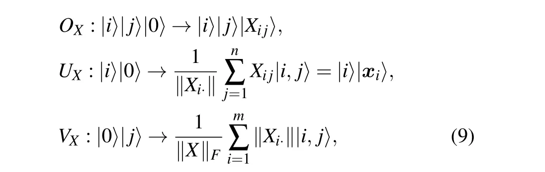
whereXi·is thei-th row ofX,i.e.,xi.

3.1.1. Algorithm details

We adopt the quantum amplitude estimation[38]and amplitude amplification[2,38]to get the neighbors ofxi. The algorithm can be decomposed into the following two stages:

Stage 1 Prepare the following quantum state by quantum amplitude estimation,

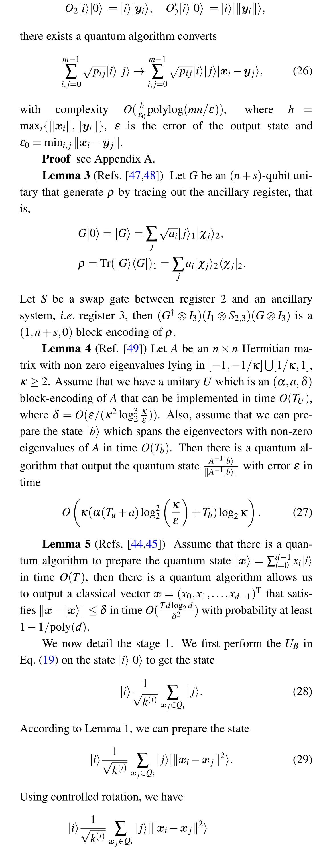
3.2. Quantum algorithm to obtain the weight matrix W

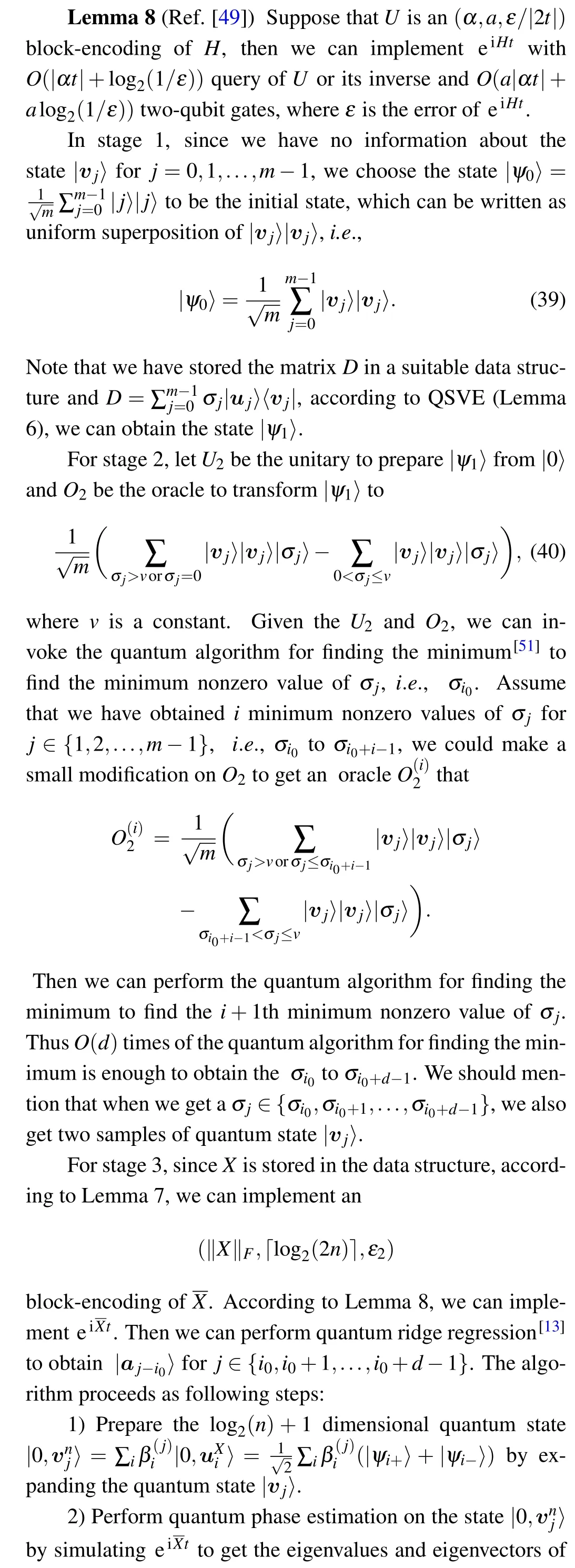
3.3. The quantum algorithm to compute the transformation matrix A

We have obtained the classical information ofWin the above algorithm. Thus we can store the information of the matrixD=I-Win a data structure that allows the following two mappings:

3.4. The total complexity and discussion

The procedure of the quantum NPE algorithm can be summarized as follows:

Algorithm 2 The procedure of quantum NPE Input: The data matrix X is stored in a data structure;Output: The quantum states|a0〉,|a1〉,...,|ad-1〉which represent each row of matrix A;1: Prepare 1 m ∑m-1i,j=0|i〉|j〉|■K m2〉;2: Prepare 1■K ∑m-1i=0 |i〉∑xj∈Qi|j〉;3: Measure the output in computational basis for several times to obtain the index j of the neighbors of xi for i=0,1,...,m-1;4: Construct oracle UB and VB;5: Prepare|ψ(i)〉to obtain ρC(i);6: Prepare|Wi〉=ρ-1 C(i)|Bi〉for i=0,1,...,m-1;7: Perform quantum state tomography on|Wi〉to get the information of Wi for i=0,1,...,m-1;8: Perform quantum singular value estimation to get|ψ1〉;9: Use the quantum algorithm for finding the minimum to find the bottom d nonzero eigenvalues and eigenvectors of M;10: Perform quantum ridge regression to get|aj〉for j=0,1,...,d-1.11: return|a0〉,|a1〉,...,|ad-1〉.

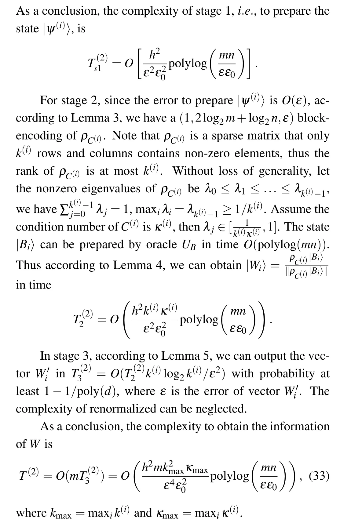
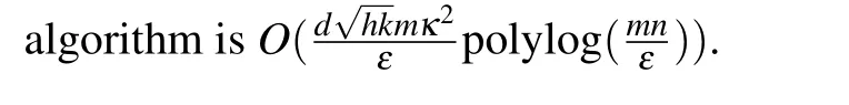
The quantum algorithm can be divided into three subalgorithms and the complexity of each sub-algorithm can be seen in Table 1. The algorithms 1–3 in Table 1 are the quantum algorithm to find the nearest neighbors, the algorithm to obtain the weight matrixWand the algorithm for embedding,respectively.h=maxi‖xi‖,k=Θ(k(i)),k(i)is the number of neighbors ofxi,mis the number of training data points,nis the dimension of the data points,εis the error of the algorithm,ε0=mini j‖xi-xj‖,kmax=maxi k(i),κmax=maxi κ(i),κ(i)is the condition number of the neighborhood correlation matrixC(i),dis the dimension of the low-dimensional space,κis the condition number of train data matrixX. Putting it all together,the complexity of the quantum NPE algorithm is

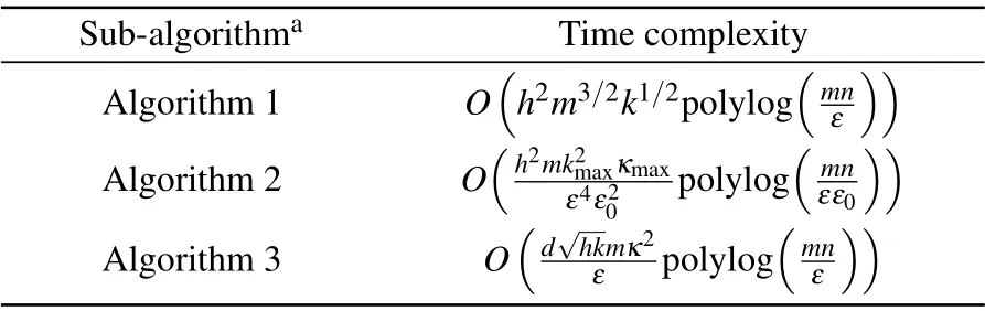
Table 1. The time complexity of the three sub-algorithms of the quantum NPE.

Since the classical algorithm have complexityO(mnk3+dm2), our algorithm have a polynomial speedup onmand an exponential speedup onnwhen the factorsd,h,kmax,κmax,ε,ε0=O[polylog(mn)]. We should mention that the output of the quantum NPE algorithm is a matrixA=(|a0〉,|a1〉,...,|ad-1〉) with each column outputted as a quantum state.

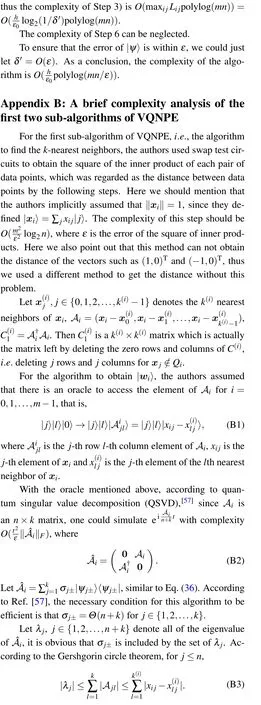
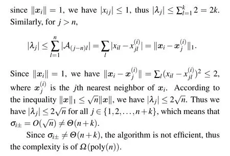
Our algorithm has two advantages over VQNPE.(i)Our algorithm is complete while VQNPE is not. In Ref.[29], the authors pointed out that it is not known how to obtain the input of the third sub-algorithm from the output of the second sub-algorithm. Actually,if just consider the completeness,we can use a VQA technique shown in Ref.[52]after our second sub-algorithm. (ii) The complexity of our algorithm is less than the complexity of VQNPE,even without considering the complexity of the third sub-algorithm of VQNPE.Specifically,The complexity of the first sub-algorithm isO(m2ε2log2n),and the complexity of the second sub-algorithm isΩ(poly(n))(we should mention that the complexity showed here are different with the original paper,see Appendix B for details),while the total complexity of our algorithm isO(m1.5polylog(mn))(only consider the main parameters). The advantage of our first sub-algorithm is mainly coming from the parallel estimation of the distance of each pair of data points. As for the second sub-algorithm, Lianget al. adopted the QSVD to get the|Wi〉. However,the eigenvalues ofAiare too small to satisfy the conditions to get an efficient algorithm,which causes the complexities to have polynomial dependence onn. We use a totally different algorithm to get the|Wi〉and the complexity analysis shows that our algorithm has complexity polylogarithmic dependence onn. As for the third sub-algorithm,it is hard to exam the complexity of the VQA of VQNPE, while our sub-algorithm has a rigorous complexity analysis.

Also,we notice that Chenet al.[55]proved a lower bound of quantum ridge regression algorithm. However, since their objective is to return a classical vector as the output of ridge regression while our algorithm(the ridge regression algorithm in the third sub-algorithm)generates a solution vector as a quantum state,the lower bound would not influence the complexity bound of our algorithm.

4. Conclusion

In this paper, we proposed a complete quantum NPE algorithm with rigorous complexity analysis.It was showed that whend,h,kmax,κmax,ε,ε0=O[polylog(mn)], our algorithm has exponential acceleration onnand polynomial acceleration onmover the classical NPE. Also, our algorithm has a significant speedup compared with VQNPE.

The Lemma 2 proposed an efficient method to append a quantum state generated by subtracting two vectors parallelly, which might have a wide range of applications in other quantum algorithms. Also, in the proof of the Lemma 2, we proposed a technique called parallel amplitude amplification,which may be of independent interest.We hope the techniques used in our algorithm could inspire more DR techniques to get a quantum advantage,especially the nonlinear DR techniques.We will explore the possibility in the future.

Acknowledgements

We thank Chao-Hua Yu for fruitful discussion and the anonymous referees for their helpful comments.

Project supported by the Fundamental Research Funds for the Central Universities (Grant No. 2019XD-A01) and the National Natural Science Foundation of China (Grant Nos.61972048 and 61976024).

Appendix A:The proof of Lemma 2 The parallel quantum amplitude amplification consists of three steps: