Lei SHI (石磊) Longxing QI (齐龙兴) Sulan ZHAI (翟素兰)

School of Mathematical Sciences，Anhui University，Hefei 230601，China E-mail:1325180014@qq.com;qilx@ahu.edu.cn;sulanzhai@gmail.com

Abstract This paper studies a kind of non-autonomous respiratory disease model with a lag effect.First of all，the permanence and extinction of the system are discussed by using the comparison principle and some differential inequality techniques.Second，it assumes that all coefficients of the system are periodic.The existence of positive periodic solutions of the system is proven，based on the continuation theorem in coincidence with the degree theory of Mawhin and Gaines.In the meantime，the global attractivity of positive periodic solutions of the system is obtained by constructing an appropriate Lyapunov functional and using the Razumikin theorem.In addition，the existence and uniform asymptotic stability of almost periodic solutions of the system are analyzed by assuming that all parameters in the model are almost periodic in time.Finally，the theoretical derivation is verified by a numerical simulation.

Key words respiratory disease;lag effect;periodic solution;almost periodic solution;Lyapunov functional

1 Introduction

The issue of air pollution has attracted great public attention on account of the continuous and large-scale haze has that spread to nearly 20 provinces and regions in China since 2013.Pulmonary particulate matter (PM2.5) is the chief culprit involved with haze pollution.PM2.5inhaled by the human body may cause respiratory diseases.Therefore，it is necessary to study the impact of PM2.5on human respiratory diseases.In recent years，many scholars have carried out investigations on this，and abundant research results have been obtained[1-4].In the above studies literatures，there is little on the use of autonomous or non-autonomous differential equation models to study the impact of air pollution on public health.Our paper will establish a non-autonomous differential equation model to examine the in fluence of PM2.5and an associated lag effect on human respiratory diseases based on the above situation.

So far，there have been few studies on the in fluence of air pollution on people’s health using the differential equation model.Most studies examine the impact of air pollution (such as haze，etc.) on people’s health according to the actual data (see[5]).In this paper，children’s respiratory diseases caused by PM2.5are taken as the research objects.Considering that sensitive people exposed to air will become sick after inhaling PM2.5，and there is no infectivity for other sensitive people，the relevant biological mathematical model is established for specific analysis.

It is generally advisable to use an autonomous mathematical model to study the impact of disease on human health，but this ignores the material fact that the correlation coefficient in such models is not always a fixed constant，but rather a function that may change with time and season.In order to make up for this deficiency，many scholars have done a great deal of research on the non-autonomous disease systems with time-varying coefficients，which has made the theoretical study on the non-autonomous differential equation model develop rapidly[6-10].The non-autonomous mathematical model is different from the autonomous in that，it has no equilibrium.As such，the persistence，extinction，existence and stability of periodic solutions and almost periodic solutions of the non-autonomous model are important areas of research，which is conducive to controlling the relevant parameters of the model to make the disease tend to extinction.

As is widely known，environmental factors fluctuate with the seasons.Therefore，some scholars study the influence of time-varying coefficient on the dynamic behavior of related population ecology models by constructing non-autonomous differential equation models[11-14].Similarly，the spread of air pollution diseases also presents some periodic characteristics with seasonal changes.For example，air pollution related diseases are widespread in the spring and winter when air pollution is relatively serious.Meanwhile，air pollution related diseases are alleviated in the summer and autumn when air pollution is relatively light.Under normal conditions，people will bring time-dependent periodic parameters into the mathematical model in order to study the influence of seasonal factors on the biological population models[15-18].Inspired by this，the periodic function of seasonal variation is drawn into the non-autonomous differential equation model，and the non-autonomous respiratory disease model with periodic parameters is set up to study the existence and attractivity of periodic solutions of the system.

Many scholars also introduced a lag effect in the process of studying the periodic solution of the non-autonomous model，so it is essential to use a non-autonomous periodic differential equation in order to study the influence of the lag effect on respiratory disease so as to more realistically reflect nature.A good deal of work has been done on the dynamic behavior of delay differential equations with periodic parameters in recent years[19-21].Among this work，there is more research on the non-autonomous model with lag effect in the theoretical research，but less in the practical，ecological or medical.On the basis of much previous research，this paper intends to establish a mathematical model of a non-autonomous periodic parameter differential equation with lag effect for the sake of studying the influence of the lag effect on respiratory disease.

One of the basic problems in studying non-autonomous functional differential equations concerns the asymptotic behavior of the system solution，and factors such as boundedness，permanence，extinction，periodicity，almost periodicity，etc..The theory of periodic solutions is also undoubtedly a significant topic in the theoretical research on functional differential equations，and scholars have attached great importance to this for many years.The most familiar research methods include topological degree theory，various fixed point theorems，monotone half flow theory，bifurcation theory，Lyapunov’s second method，and critical point theory，etc.[22-24].This paper intends to testify to the existence of a periodic solution for a non-autonomous respiratory disease model by using the continuation theorem from the coincidence degree theory by Mawhin and Gaines，and to analyze the global attractivity to periodic solution of the model by constructing the appropriate Lyapunov functional.

Periodic fluctuations of the environment play an important role in many biological and ecological dynamic systems in the natural world.Therefore，parameters that are almost periodic in the natural environment should be considered if some parameters in the model are not a periodic function of an integral multiple and we have no prior knowledge that these time-varying parameters must be periodic as part of the procedure of integrating the seasonal environmental factors into the conventional mathematical model.Ever since Bohl established the system theory of almost periodic functions in the 1920s，theoretical research on the almost periodic function has received a lot of attention from scholars as a kind of extension of the periodic function，and this research has developed quickly.Many scholars have demonstrated that it is more realistic to adopt an almost periodic hypothesis in the process of almost periodic study，when taking into account the impact of environmental factors，and this has certain ergodicity[25-30].At present，most studies on the almost periodic solutions of differential equation models focus on purely theoretical analysis，but lack the practical work of combining the theory with the actual biomedical background.Therefore，this paper will study the existence and stability of an almost periodic solution of a non-autonomous respiratory disease model that integrates of the authentic background.

In other words，there is much literature on respiratory disease based on the actual monitoring data，but little on the periodic or almost periodic situation that uses a differential equation model.An autonomous respiratory disease model with lag effect was established based on actual monitoring data，and the local，global stability and Hopf bifurcation of the model were studied in[31].However，the non-autonomous case of this model is not considered in the literature cited above.Therefore，in this paper a non-autonomous respiratory disease model with lag effect is proposed in order to study the persistence and extinction，and the existence and global attraction of periodic solutions，and the existence and stability of almost periodic solutions.

The structure of this paper is as follows:Section 2 is an introduction to the non-autonomous respiratory disease model with a lag effect.In Sections 3 to 6，the persistence，extinction，existence and global attraction of periodic solutions，and the existence and uniform asymptotic stability of almost periodic solutions are analyzed.In Section 7，a numerical simulation is conducted.Finally，a conclusion and discussion are presented.

2 Non-autonomous Respiratory Disease Model with Lag Effect

First，there is much literature on the impact of air pollution on people’s health，most of which considers the situation in which patient groups transmit disease to susceptible people[32-35].Mathematical modeling is carried out in this paper based open the phenomenon of the groups directly becoming patients after inhaling PM2.5，without patients being contagious to other sensitive people.

Second，the prevalence of respiratory diseases depends not only on the current state，but also on the previous state.Under normal circumstances，morbidity is likely to occur with time delay，as diseases have a complicated evolutionary process[36-38，40-43].For respiratory diseases，is possible that sensitive parts of a population exposed to polluted air may not show symptoms immediately after inhaling PM2.5，yet become patients at a later time.

Thus，it is of great practical significance to study the non-autonomous mathematical model with time-varying coefficients，as the parameters of the air pollution-related disease model may change significantly with time[6-10，13-15，39，40].Based on the three practical problems noted in the above，and using the classical methods and analysis techniques of the non-autonomous infectious disease model，this paper intends to establish a non-autonomous respiratory disease model with a lag effect and without infectivity to carry out a theoretical analysis with the intention of getting more practical research results.

In accordance with the general understanding，this paper makes the following two assumptions:1) Suppose that natural death occurs in both sensitive groups and patients，that patients have mortality from illness，and that patients could recover to join the sensitive population after treatment;2) Denote the time (the lag days in the body of patients) between a subject’s exposure to PM2.5and becoming patients as a constant τ，so that sensitive people exposed at time t-τ will become patients at time t.Based on this，the model of non-autonomous respiratory diseases with a lag effect is constructed as follows:

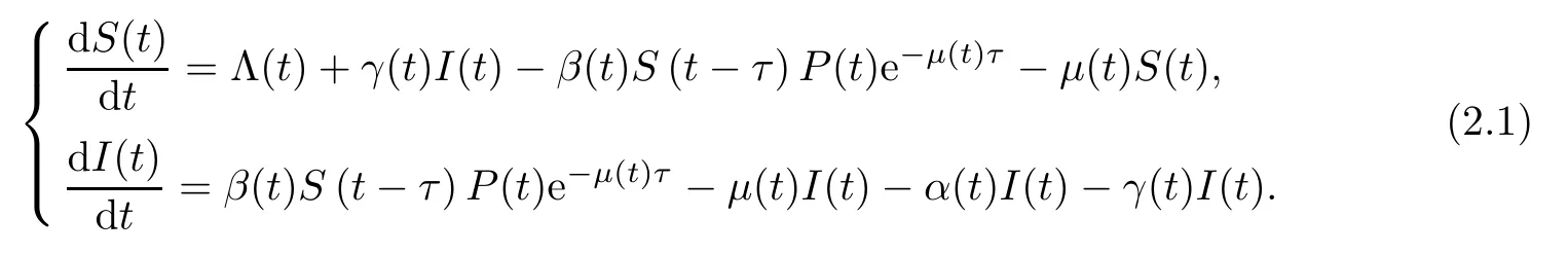
Here S (t) and I (t) represent the number of susceptible groups and patients at time t，respectively.The parameter Λ(t) is the recruitment rate function of susceptible groups;P (t) denotes the air pollution index at time t;μ(t) is the natural death rate function of susceptible groups and patients;β(t) is the conversion rate function of air pollution exposure of patients per unit of time;α(t) is the disease-induced death rate function of patients;and γ(t) is the cure rate function of patients.The item β(t) S (t-τ) P (t) indicates the number of susceptible groups that inhaled PM2.5at time t-τ，and the item β(t) S (t-τ) P (t) e-μ(t)τdenotes the number of patients showing symptoms at time t.

In terms of practical applications，we focus our discussion on positive solutions of system (2.1).It is assumed that system (2.1) has initial conditions

where φ(θ)，φ(θ) is the continuous function of a nonnegative bounded on θ∈(-τ，0].

This paper assumes that the coefficients of system (2.1) are all continuous，strictly positive functions，and are bounded above and below by positive constants on (-∞，+∞).We also made the following remark:

3 Persistence

Definition 3.1([41，42]) The system (2.1) is persistent if there exists a compact region D⊂|S≥0，I≥0}such that every solution (S (t)，I (t))Tof system (2.1) will ultimately enter and stay in the compact region D all the time.

Lemma 3.2([41-43]) Let a＞0，b＞0.If

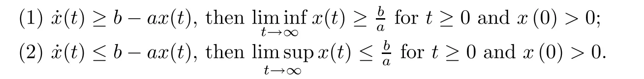
Lemma 3.3([41，44]) Suppose a＞b＞0，c＞0，x (0)＞0.Then if

Lemma 3.4([41，44]) Considering the equation

with (a，b，c，τ＞0，x (t)＞0for-τ≤t≤0)，one has that

(2) if a＜b，then x (t)=0.

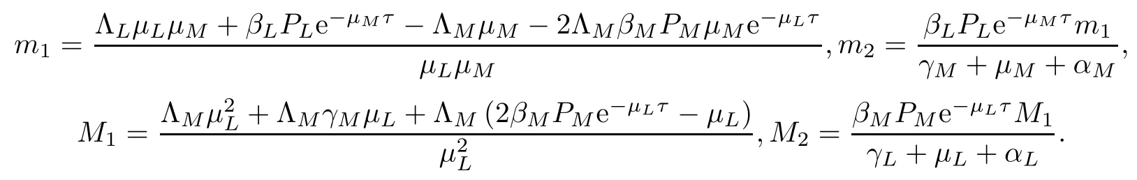
Theorem 3.5Suppose that system (2.1) has an arbitrary solution (S (t)，I (t))Tsatisfying the initial condition (2.2).Assume further that the system (2.1) satisfies the following inequality:

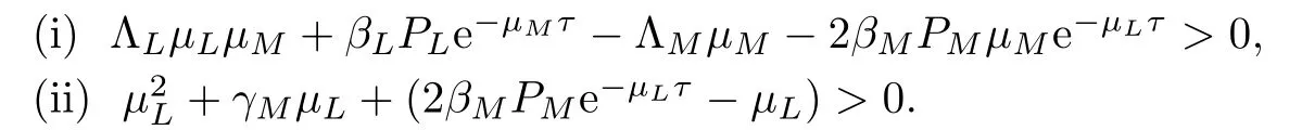
Then there exist T′＞0 and T′′＞0 such that S (t)≥m1，I (t)≥m2，S (t)≤M1，I (t)≤M2.Therefore the system (2.1) is persistent，where

ProofAccording to the mathematical modeling and the practical application background regarding the non-autonomous respiratory disease model，it can be obtained that

owing to the fact that

N′(t)=S′(t)+I′(t)=Λ(t)-μ(t)(S (t)+I (t))-α(t) I (t)≤Λ(t)-μN (t)，

When T1＞0，the following formula is obtained from the first equation of system (2.1):

In light of Lemmas 3.3 and 3.4[41，44]，in the case that＞μM，we have

Substituting formula (3.2) into equation (3.1)，and from the application of Lemma 3.2[41-43]，it can be seen that

when t＞T1+τ.Here，we choose

In line with the second equation of system (2.1)，it can be obtained that

when t＞T2.

Referring to Lemma 3.2 in references[41-43]，there exists t＞T2+τ，and setting m2=，we can get

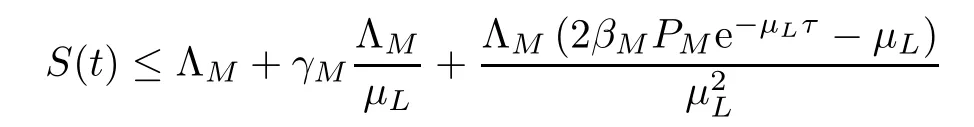
We have

if t＞T′，and we select T′=max{T1，T2}.

On the other hand，again from the first equation of system (2.1)，it can be obtained that

when t＞T3.

On the basis of Lemmas 3.3 and 3.4[41，44]，it can be obtained that

Substituting formula (3.6) into expression (3.5)，by Lemma 3.2[41-43]it can be found that

if t＞T3+τ.We choose that

Grampy held my hand tightly. Together we looked up the street and down, and back up again. He stepped off the curb and told me it was safe to cross. He let go of my hand and I ran. I ran faster than I had ever run before. The street seemed wide. I wondered if I would make it to the other side. Reaching the other side, I turned to find Grampy. There he was, standing11 exactly where I had left him, smiling proudly. I waved.

As a result of the second equation of system (2.1)，it can be obtained that

when t＞T4.

From Lemma 3.2[41-43]we get that

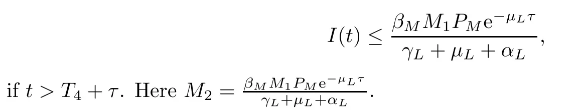
Letting T′′=max{T3，T4}，one has that

if t＞T′′.Therefore，there is a compact region

which is the uniformly bounded set of system (2.1) if

According to the discussion above，every solution of system (2.1) with initial value condition (2.2) will enter and finally stay in the compact region if equations (3.9) and (3.10) are satisfied.Then，by the Definition 3.1 in this section system (2.1) is persistent. □

4 Extinction

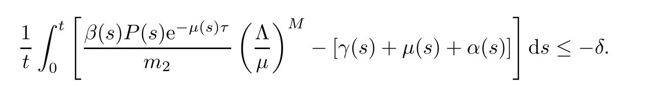
Theorem 4.1Suppose that for arbitrary ε＞0 there is a positive constant δ＞0 such that

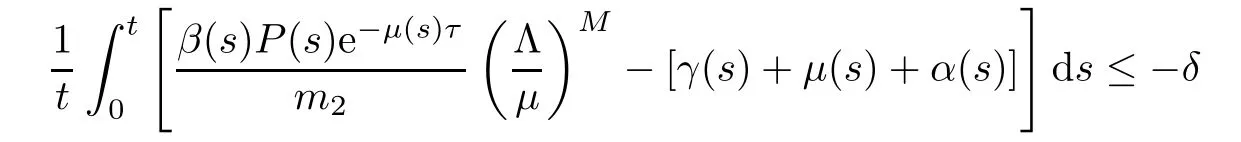
for any t≥ε.As a resut，patients I (t) are extinct;that is to say，=0.

ProofFrom N*(t)=S (t)+I (t)，system (2.1) can be converted to

For the first equation of system (4.1)，one has that

Therefore，by Lemma 3.2[41-45]，it can be seen that

From the second equation of system (4.1)，it can be known that

For any t≥ε＞0，by integrating both ends of (4.2) from 0 to t，it can be obtained that

Thus it can be seen that if=0，the patients I (t) are extinct. □

From the above，it can be seen that in order to prove that the disease has been made extinct，what we have to do is to prove that the solution of the function I (t)，regarding the number of patients，is zero or of negative growth all the time.In the proof of Theorem 4.1，we have proven that the solution curve of the function I (t) presents negative exponential growth，so the solution of the function I (t) will eventually tend to zero.In this way，the number of patients will go to zero，and the air pollution related disease will die out.

5 Positive Periodic Solution

5.1 Existence of positive periodic solutions

In this section，we assume that all coefficients Λ(t)，β(t)，P (t)，γ(t)，μ(t)，α(t) of system (2.1) are strictly positive T-periodic continuous functions on R+=[0，∞)，so system (2.1) becomes a T-periodic system.Based on the continuation theorem from the coincidence degree theory of Mawhin and Gaines[41，42]，we will demonstrate that system (2.1) has at least one positive periodic solution.First of all，the Definition and Lemma needed for the proof are introduced.

Definition 5.1([41-46]) Hypothese X，Y are normed vector spaces，G:DomG⊂X→Y is a linear map，Z:X→Y is a continuous map.The mapping G is the Fredholm mapping with zero index if ImG is a closed subset of Y and KerG=condimImG＜+∞.

Suppose the mapping G is the Fredholm mapping with zero index if ImG is a closed subset of Y.Then there is projection mapping E:X→X，F:Y→Y such that ImE=KerG and ImG=Ker F=Im (I-F) is established.Thus the mapping

G|DomG∩KerE:(I-E) X→ImG

is invertible，and its inverse mapping is KE.

Let us suppose that Ω is a bounded open subset of X，that the map Z is called G-compact on，thatis bounded and that KE(I-F) Z:→X is compact.Also，because ImF and KerG are isomorphisms，there is an isomorphism mapping J:Im F→KerG[41-46].

Lemma 5.2(Continuation theorem[41-46]) Assume that the mapping G is the Fredholm mapping with zero index，and the mapping Z is called G-compact on.Assume also the following conditions:

Then，Gx=Zx has at least one solution on∩DomG.

If f (t) is a continuous function with period T，then we have

Theorem 5.3Suppose that the conditions

are satisfied.Then system (2.1) has at least one positive T-periodic solution.

ProofLet g1(t)=lnS (t)，g2(t)=lnI (t).The system (2.1) can be written as follows:

and denote the projections E and F as follows:

It is easy to see that KerG=R2，ImG=closed in Y，and that dimKerG=2=codimImG.At the same time，E，F are continuous projection operators and ImE=KerG，KerF=ImG=Im (I-F).

Hence，the mapping G is the Fredholm mapping with zero index，and its inverse mapping KE:ImG→DomG∩KerE has the following form:

What is clear is that FZ，KE(I-F) are continuous，so we can get thatis bounded，and KE(I-F)is tight on the bounded open set Ω⊂X，by the Arela-Asili theorem[41-45].Therefore，Z is T-close on.

Corresponding to operator equation Gg=σZg (0＜σ＜1)，one has

Let g∈X be the solution of system (5.2).Then there exists φi，φi∈[0，T]，which gives

Obviously gi′(φi)=gi′(φi)=0，i=1，2.It can be seen that

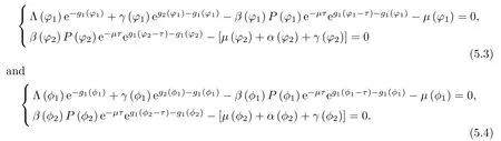
Therefore，it can be obtained，from the first equation of the system (5.3)，that

In accordance with the second equation of system (5.3)，it can be seen that

On the basis of the first equation of system (5.4)，we have that

Again，from the second equation of system (5.4)，one has that

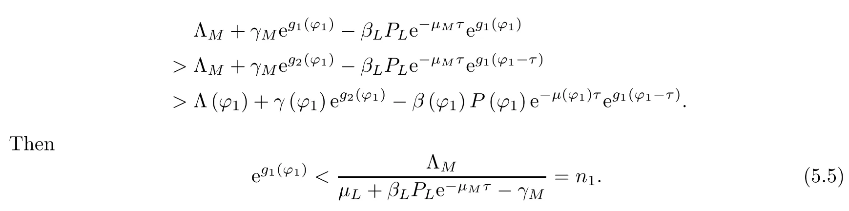
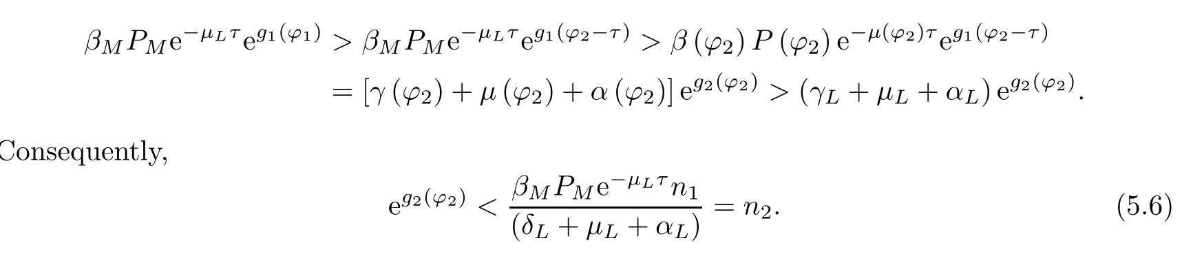
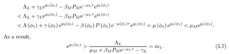
It can be seen from this that one acquires

Moreover，we have obtained that

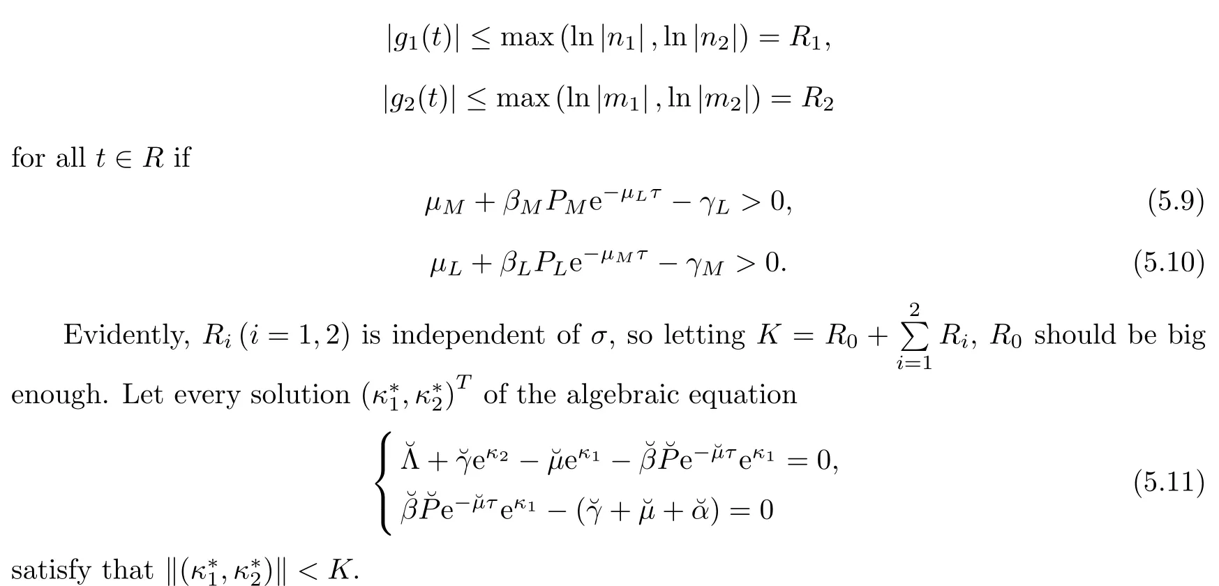
if g∈∂Ω∩KerΩ=∂Ω∩R2，and=K，with g being the constant vector in R2.Thus condition (b) of Lemma 3.2 in reference[41]is obtained，at this corresponds to condition (ii) of Lemma 5.2.

Finally，we certify that the condition (c) of Lemma 3.2 in reference[41]is tenable，at this corresponds to the condition (iii) of Lemma 5.2.From the algebraic equation

Hence，it can be seen，from the theory of topological degree[41-46]，that

In view of this，three conditions of Lemma 3.2 from[41](Lemma 5.2 in this paper) have been proved.Therefore，the system (5.1) contains at least one periodic solution if equations (5.9) and (5.10) are satisfied.Thus，system (2.1) has at least one positive T-periodic solution. □

5.2 Global attraction of positive periodic solutions

Definition 5.4([41-48]) Suppose that (S*(t)，I*(t))Tis the positive periodic solution of system (2.1)，and let (S (t)，I (t))Tbe any positive solution of system (2.1).Then the periodic solution (S*(t)，I*(t))Tof system (2.1) is attractive if

Lemma 5.5([41-48]) Suppose that η is any positive constant，and that f is a nonnegative function defined on interval[η，+∞).Then we have=0 if f is integrable and uniformly continuous in interval[η，+∞).

Theorem 5.6The positive periodic solution (S*(t)，I*(t))Tof the system (2.1) is globally attractive if system (2.1) satisfies the conditions of Theorem 3.5，Theorem 5.3 and the following inequalities:

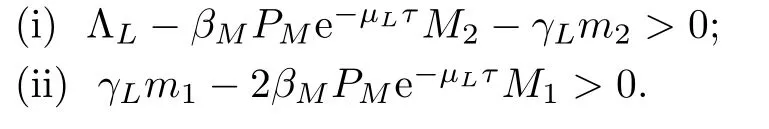
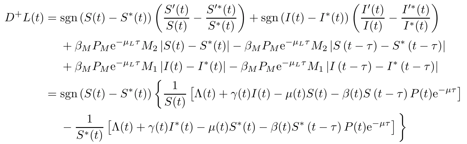
ProofFirst，the following Lyapunov functional is constructed[41，45-48]:

Then，by calculating the upper right derivative of function V along the positive solution of system (2.1)，we get that

On the other hand，from Theorem 3.5，we get that

m1≤S (t)≤M1，m2≤I (t)≤M2.

Thus，it can be obtained that

Therefore，by taking the above (5.13) and (5.14) into (5.12)，it can be obtained that

According to the Razumikin theorem given in literatures[45-48]，and the integral on interval[T，t]from the above inequality (5.15) for any t≥T，it can be seen that

Then|S (t)-S*(t)|∈L1[T，+∞)，|I (t)-I*(t)|∈L1[T，+∞).

It can be acquired，from system (2.1) and Theorem 3.5，that S (t)，I (t) and S′(t)，I′(t) are bounded on the interval[T，+∞).This shows that|S (t)-S*(t)|and|I (t)-I*(t)|are uniformly bounded in interval[T，+∞).

In conclusion，the positive periodic solution of system (2.1) is globally attractive. □

6 Almost Periodic Solution

The almost periodic solution is a more common phenomenon than the periodic solution and to a certain extent contains the results of periodic situation.For describing the population ecology dynamics model subjected to seasonal climate and other environmental factors，the situation of an almost periodic solution is undoubtedly closer to reality.It is of great practical significance to study the almost periodic problem on a time scale for the purpose of researching of biological and ecological models changing with time[48-52].We assume that all the coefficient functions Λ(t)，β(t)，P (t)，γ(t)，μ(t)，α(t) of system (2.1) are almost periodic，so system (2.1) is called an almost periodic system.

Definition 6.1([50-52]) If there is a constant δ(ε)＞0 for any ε＞0，such that there exists τ＞0 in any interval of δ(ε)＞0，and the inequality|f (t+τ)-f (t)|＜ε holds for all t∈(-∞，+∞)，then the function f (t) is almost periodic.

Lemma 6.2([50-52]) Consider the system

and its product system

Theorem 6.3Suppose that the almost periodic system (2.1) satisfies the inequalities

Then system (2.1) has an almost periodic solution which is of uniform asymptotic stability in Ω.Here Ω={(S (t)，I (t)):m1≤S (t)≤M1，m2≤I (t)≤M2}is the ultimately bounded positive invariant set of system (2.1).

ProofLet us first consider the product system associated with system (2.1)[50-54]:

We suppose that (X (t)，Y (t))∈Ω×Ω is the solution of system (6.1)，and

X (t)=(S (t)，I (t))，Y (t)=(S1(t)，I1(t)).

Next，the following parameter transformation is done:

Then，the solution of the product system corresponding to system (2.1) that can be obtained is

That is to say，the solution of the product system associated with system (2.1) is

Then，the continuous non-subtractive Lyapunov function is constructed:

In addition，we prove one by one that the functions satisfy the three conditions of the existence and uniform asymptotic stability of almost periodic solutions[50-54].

First，it can be obtained that ξL (t)≤L (t)≤ηL (t)，and ξ=min，η=max.Letting a (s)=ξ(s)，b (s)=η(s)，one has that a (s) L (t)≤L (t)≤b (s) L (t)，where a (s)，b (s) is continuously monotonically increasing and positive definite.Therefore，function L (t) satisfies the first condition for the existence and uniform asymptotic stability of almost periodic solutions[50-54].

This proves that function L (t) satisfies the second condition for the existence and uniform asymptotic stability of almost periodic solutions[50-54].

Then，taking the continuous and non-subtractive function Q (s)=(1+ε) s＞s for any ε＞0，we have that

Next，the upper right derivative of L (t) along the product system (6.1) is calculated as follows:

It can seen，from Theorem 3.5，that S (t)≥m1，I (t)≥m2.This can also be seen because

Therefore，

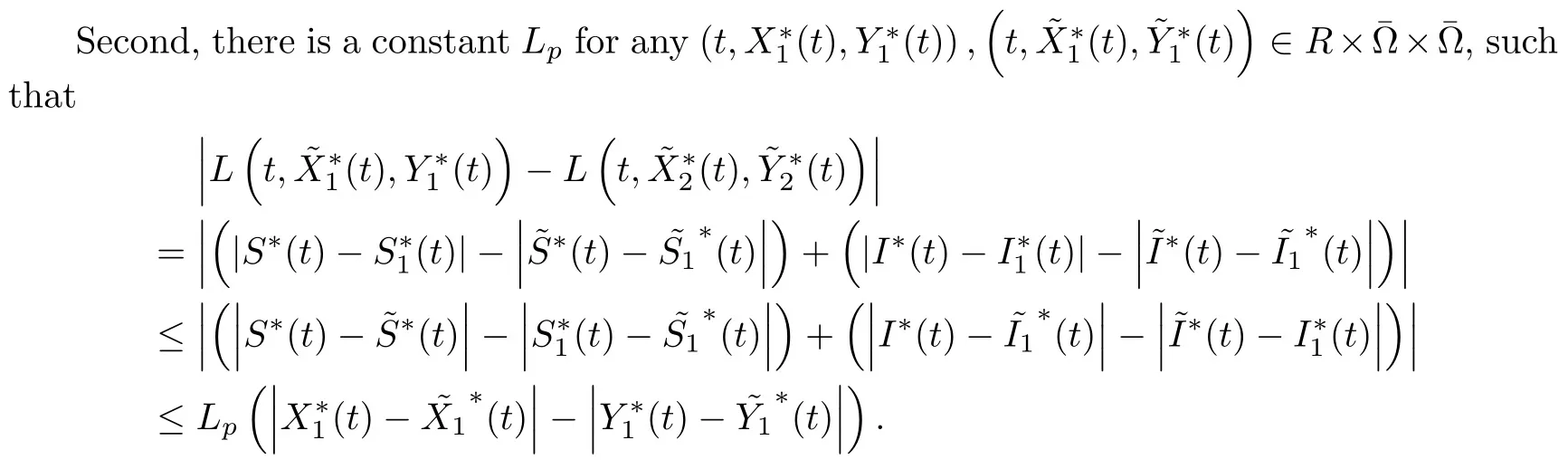
In addition，according to the differential mean value theorem[50-54]，there exists ζi(i=1，2)，which gives that

In line with formula (6.2)，it can be found that

Putting formula (6.4) into equation (6.3) we get

we get that

So far，has been proven that function L (t) satisfies three conditions for the existence and uniform asymptotic stability of almost periodic solutions[50-54].Therefore，system (2.1) has an almost periodic solution and which has uniform asymptotic stability. □

7 Numerical Simulation

In this section，a non-autonomous respiratory disease model with a lag effect will be simulated.According to the actual monitoring data of the air pollution index for Hefei city in the Anhui Province in 2016(on the official website of China Meteorological Administration)，the function expression P (t) of PM2.5is obtained by numerical fitting as follows:

7.1 Periodic solution

In accordance with the proof process outlined in Sections 5.1 and 5.2，the system has at least one positive periodic solution if the time-varying parameters of system (2.1) meet the relevant conditions of Theorem 5.3.The positive periodic solution of the system is globally attractive in the case where the time-varying parameters of system (2.1) satisfy the conditions of Theorem 5.6.

The parameters of model (2.1) in the process of numerical simulation are as follows[8，31，38，42，43，51-59]:

The positive periodic solution of system (2.1) is demonstrated in Fig.1 for when the lag day τ is 1，2，3，4，5 in turn.The numerical simulation of Fig.1 verifies the theoretical derivation shown in Sections 5.1 and 5.2.It shows that there is a positive periodic solution of system (2.1) which is globally attractive if certain parameters and conditions of the model are satisfied.In addition，the simulation shows that the variation magnitude of the number of patients I (t)，increases with the rise in lag days from 1 to 5，and the top peak value of I (t) is smaller and smaller.Meanwhile，the variation magnitude of susceptible group’s number，S (t)，decreases with the rise in the lag days，and the top peak value of S (t) is bigger and bigger.

Figure 1 Periodic solution of system (2.1) with different lag days τ=1，τ=2，τ=3，τ=4，τ=5 in susceptive groups and patients in Fig.1a and Fig.1b，respectively.

7.2 Almost periodic solution

According to the proof of Theorem 6.3，system (2.1) will have an almost periodic solution similar to the periodic form if the parameter value of system (2.1) satisfies the two conditions of Theorem 6.3.This almost periodic solution has uniform asymptotic stability at the mean time，and which is uniformly stable and uniformly attractive.

On the basis of the ε-δ definition of the uniform asymptotic stability of solutions to differential equations，with the uniform asymptotic stability of almost periodic solutions of differential equations it doesn’t matter what the initial values of the system are.That is to say，the almost periodic solution of system (2.1) has uniform asymptotic stability regardless of the initial values (S0，I0).A numerical simulation is now used to verify these theoretical results.

The parameters used in the process that depicts almost periodic solutions are as follows[8，31，38，42，43，51-59]:

From the numerical demonstrated in Fig.2，it can be seen that the different initial values of the sensitive population S0and the sick population I0have no effect on the uniform asymptotic stability of the almost periodic solution of system (2.1).If the initial value of the sensitive population increases from 70000 to 110000，and the initial value of the sick population increases from 11000 to 51000，then the numbers for the sensitive population S (t) and the sick population I (t) will appear to be almost periodic oscillations in periodic form.Finally，this tends to be uniformly stable and uniformly attractive.It is proven that the almost periodic solution of system (2.1) has uniform asymptotic stability，and the theoretic derivation of Theorem 6.3 in this paper is proven more forcefully.

Figure 2 The almost periodic solution of system (2.1) with different initial values (70000，11000)，(80000，21000)，(90000，31000)，(100000，41000)，(110000，51000) in the sensitive and the patients populations，when τ=5.

From Fig.3，as the lag time τ increases from 3 to 7，it is found that the oscillation amplitude of the almost periodic solution produced by the patients’number I (t) increases slowly，and the top peak value of the change of I (t) decreases gradually.However，the susceptible groups number S (t) decreases slowly，and the top peak value of the change of S (t) increases gradually.

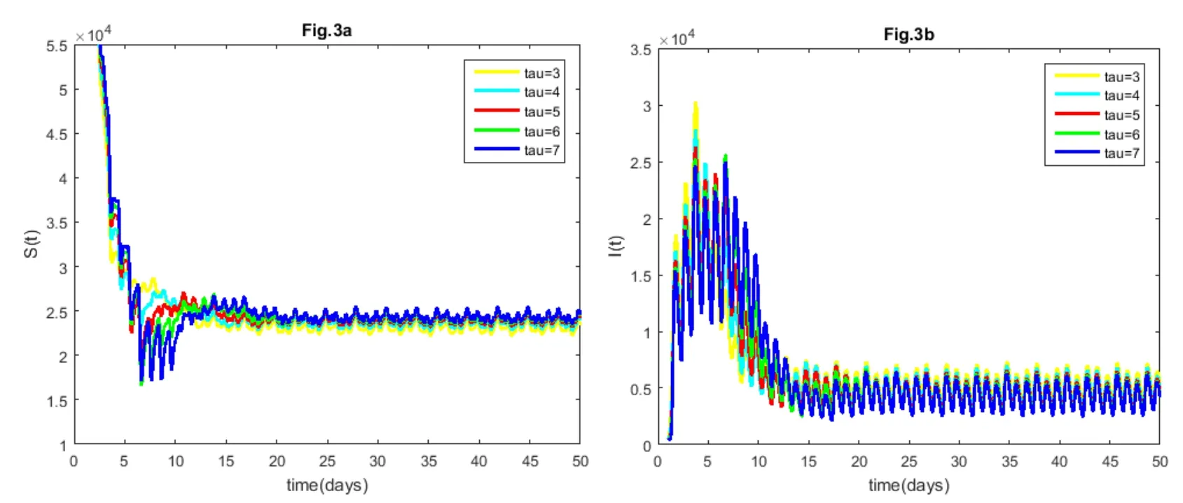
Figure 3 Almost periodic solutions of system (2.1) with different lag days τ=3，τ=4，τ=5，τ=6，τ=7 for susceptible groups and patients in Fig.3a and Fig.3b，respectively.

8 Conclusion and Discussion

Based on the transmission mechanism of respiratory diseases，the actual biological background of susceptible people getting sick directly after inhaling air pollutants has been considered.A non-autonomous respiratory disease model with a lag effect has been established.The permanence and extinction of the system have been discussed，the existence and global attractivity of positive periodic solutions of the system have been proved，and the existence and uniform asymptotical stability of almost periodic solutions of the system have been obtained.At the same time，this paper has also studied the impact of lag days on respiratory diseases by combining theory with the actual data.This research has aimed to provide some help for people to understand the pathogenesis of respiratory diseases from the theoretical perspective，with a good practical application value.

Synthesizing the theoretical analysis results from Sections 3 to 6 of this paper，it has been found that the conditions of the persistence，the existence and global attraction of positive periodic solutions，and the existence and uniform asymptotical stability of almost periodic solutions of the system (2.1) are closely related to PM2.5and the number of lag days，τ，in patients.Then，the relationship between PM2.5，lag days τ and the permanence，the existence and global attraction of positive periodic solutions，existence and uniform asymptotic stability of almost periodic solutions of system (2.1) have been discussed.

According to the first condition of Theorem 3.5，we obtained that

Based on the second condition，we have seen that τ2＜.Calculating by the parameter values，one has that τ1＜13，τ2＜23.Thus，we have τ＜min (τ1，τ2)=13.It can be concluded that the number of sensitive and of patients in the system (2.1) are persistent when the lag days for patients is less than 13.

From the first condition of Theorem 5.3，we obtained that τ1＜.According to the second condition，we have that τ2＜.By choosing appropriate parameter values，it has been obtained that τ1＜6，τ2＜9.Therefore，one has that τ＜min (τ1，τ2)=6.It can be concluded that there is at least one positive periodic solution of the system (2.1) where the lag days for patients is less than 6.

In the light of the first condition in Theorem 5.6，we obtained that τ1＞.From the second condition，one has that τ2＞，from the parameter value.Combining the appropriate parameter values，we have that τ1＞1，τ2＞2.Thus，we know that τ＞max (τ1，τ2)=2.According to Theorem 5.6 and the above analysis，the positive periodic solution (S*(t)，I*(t))Tof system (2.1) is globally attractive if the system satisfies the conditions of Theorems 3.5 and 5.3，and the lag days are more than 2.Combined with the theoretical derivation and parameter values of Theorems 5.3 and 5.6，the patients number will eventually appear to be a relatively stable periodic oscillation phenomenon when the lag days are 2＜τ＜6.

From the first condition of Theorem 6.3，it has been seen that τ1＞.For the second condition，we have discussed this in two cases:

In line with the above two lines of analysis，it has been acquired that

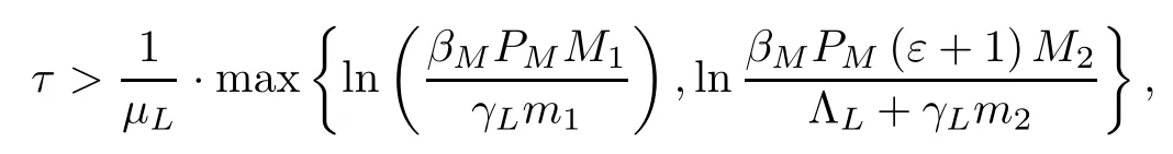
In accordance with the parameter values，one has τ1＞0.7，τ2＞1.1 or τ2＞2.1.Then τ＞max (0.7，1.1) or τ＞max (0.7，2.1).Therefore，the system (2.1) has an almost periodic solution in its ultimately bounded positive invariant set when the lag days are more than 2，and the solution is of uniform asymptotic stability.This means that there will be a relatively stable，almost periodic oscillation phenomenon similar to the periodic form in the patients number.

To sum up，the number of lag days has a great influence on the theoretical results of the non-autonomous respiratory disease model with a lag effect.The larger τ is，the smaller the amplitude of the oscillation in the patients number，and the top peak value of the change in the patients number I (t) is gradually decreases.However，the more days the disease incubates in the patient group，the more unfavorable the situation becomes for treating the respiratory disease.At the same time，the establishment of a non-autonomous mathematical model with periodic and almost periodic time-varying coefficients is helpful for studying the impact of respiratory diseases on human health more closely，and this can also enrich the theoretical research on differential equations.