Chunmao HUANG (黄春茂)

Department of Mathematics，Harbin Institute of Technology (Weihai)，Weihai 264209，China E-mail:cmhuang@hitwh.edu.cn

Chen WANG (王晨)

School of Data and Computer Science，Sun Yat-sen University，Guangzhou 510006，China E-mail:wangch329@mail2.sysu.edu.cn

Xiaoqiang WANG (王效强)†

School of Mathematics and Statistics，Shandong University，Weihai 264209，China E-mail:xiaoqiang.wang@sdu.edu.cn

Abstract Let (Zn) be a branching process with immigration in a random environment ξ，where ξ is an independent and identically distributed sequence of random variables.We show asymptotic properties for all the moments of Zn and describe the decay rates of the n-step transition probabilities.As applications，a large deviation principle for the sequence logZn is established，and related large deviations are also studied.

Key words branching process with immigration;random environment;moments;harmonic moments;large deviations

1 Introduction

As an important extension of the Galton-Watson process，the branching process in a random environment (BPRE) has received extensive attention.Smith and Wilkerson[34]introduced the concept of independent and identically distributed (i.i.d.) environment variables into the Galton-Watson process and studied the certain or noncertain extinction.Athreya and Karlin[2，3]generalized the environment variables to a more common situation called a stationary and ergodic environment，and established some basic limit theorems.A lot of asymptotic properties and behaviours of BPRE-such as limit theorems，large deviations，survival probabilities，moments and convergence rates of martingales-have been studied;see for example[6，7，9，14，15，17，18，21，24，37].

The model of the branching process with immigration in a random environment (BPIRE) extends BPRE by considering the in fluence of the immigration.Based on the original reproductive mechanism of BPRE，a certain number of alien populations join the original population at every generation.The initial conditions of the branching process can determine whether or not the population will become extinct over time.The immigration can actually also be used to prevent extinction.The latter overcomes some of the former’s limitations on variable restrictions.

After BPIRE was proposed，some scholars devoted themselves to building their theoretical framework by studying its commonalities with BPRE;see the papers[4，11，12，25，33，36，38].However，the theoretical research on BPIRE is still lacking and the relevant theories are not yet mature，which limits some applications.For example，Bansaye[4]needed to base his work on some asymptotic properties of BPIRE when he studied cell contamination models.Among the studies on BPIRE，Wang and Liu[38]established the principles of large deviation and moderate deviation for supercritical BPIRE.Based on their work，our study completes the theory of moments and improves the condition of the large deviation principle of BPIRE.For branching processes with immigration and related topics，recent developments can be found in the papers[16，26，27，32，37，39];readers may refer to the references therein for more information.

1.1 Description of the model and the notation

Let us describe the model in detail.We consider a branching process with immigration in a random environment (BPIRE).The random environment，denoted by ξ=(ξn)，is an i.i.d.sequence of random variables taking values in some measurable space Θ.Without loss of generality，we can suppose that ξ is de fined on the product space (ΘN，E⊗N，τ)，where τ is the law of ξ and N={0，1，2，···}.Each realization of ξncorresponds to two probability distributions on N:one is the offspring distribution denoted by

the other is the distribution of the number of immigrants denoted by

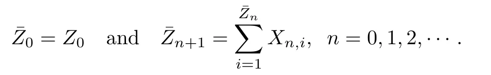
In particular，we write pi=pi(ξ0) and hi=hi(ξ0) for brevity.The branching process (Zn) with immigration Y=(Yn) in the random environment ξ is de fined as follows:the process starts with Z0initial individuals，and Z0is independent of the environment ξ.Then

where given the environment ξ，Z0，Xn，i(n=0，1，2，···，i=1，2，···) and Yn(n=0，1，2，···) are all independent of each other，Xn，ihas the distribution p (ξn) and Ynhas the distribution h (ξn).We write Xn=Xn，1for brevity.The random variable Xn，ican be regarded as the number of offspring of the i-th individual in the n-th generation and Ynas the amount of immigration in the (n+1)-th generation，so that Zn+1represents the total population of the (n+1)-th generation.If h0=1，there is no immigration and the process (Zn) forms the so-called branching process in a random environment (BPRE) which is what has been largely studied in the literature.To distinguish between BPRE and BPIRE，we useto denote the process BPRE without immigration Y，i.e.，

It is clear that Zn≥.

Let (Γ，Pξ) be the probability space on which the process is de fined when the environment ξ is given.The total probability space can be formulated as the product space (Γ×ΘN，P)，with P (dx，dξ)=Pξ(dx)τ(dξ).The probability Pξis usually called a quenched law，while the total probability P is usually called an annealed law.The quenched law Pξmay be considered to be the conditional probability of the annealed law P given ξ.Moreover，for k∈N*={1，2，···}，denote Pk(·)=P (·|Z0=k) as the probability conditioned on{Z0=k}for the process starting with k initial individuals.The expectation with respect to Pξ(resp.P，Pk) will be denoted by Eξ(resp.E，Ek).

For n∈N and t∈R，set

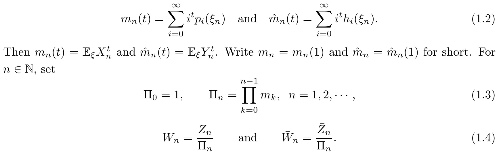
Let F0=σ(ξ) and Fn=σ(ξ，Yl，Xl，i:0≤l＜n，i≥1)，(n≥1).It is known that under the probability Pξ(·|Z0=k)，(Wn，Fn) forms a nonnegative submartingale，and it converges almost surely (a.s.) to some limit W if Elogm0＞0 and＜∞，by[38，Theorem 3.2]，while (，Fn) is a nonnegative martingale and hence it naturally converges a.s.to a limit.

Just as with the case of BPRE，the asymptotic behaviour of the process Zncan often be analysed with the help of the moments of Zn，or those of Wn.For a branching process in an i.i.d.environment，Huang and Liu studied the moments ofof positive orders in[22]and those of negative orders in[21].Wang and Liu generalized these results for a branching process with immigration in an i.i.d.environment in[38].Here，we want to investigate the annealed moments of Zn;namely，for s∈R.We remark that the quenched moments of Zncan be studied via the corresponding quenched moments of Wn，which was discussed in another paper by the authors[23].

Let us briefly introduce the structure of this article.For the rest of Section 1，we summarize the main results and conclusions.First，based on the Lpconvergence of the submartingale Wnof BPIRE studied in[38]，we show the asymptotic properties of the moments(see Theorem 1.1).Second，we describe the decay rates of the n-step transition probabilities (see Theorem 1.2) and those of the harmonic moments(see Theorem 1.5).Third，we show large deviations for logZn(see Theorems 1.7 and 1.8).Section 2 is devoted to the proof of Theorem 1.1.In Section 3，a sharp upper bound for harmonic moments is given to prepare for the proofs of Theorems 1.2 and 1.5.In Sections 4-6，the proofs of Theorems 1.2，1.5 and 1.8 are shown successively.

1.2 Main results

We first show the annealed convergence rates of the positive moments of Zn.

Theorem 1.1(Moments) Let p＞0，and assume that∈(1，∞).Then，

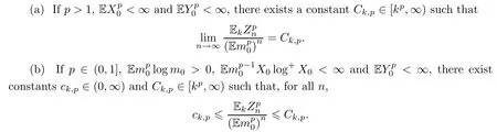
Theorem 1.1 shows that under necessary moment conditions，has the same asymptotic properties asfor p＞0.For BPRE，a similar result was shown in[21，Theorem 1.3].

Next we consider the harmonic moments of Zn.From now on we will restrict things to the case that

(H0) P (p0=0)=1 and P (p1=1)＜1.

The first condition means that each individual produces at least one child，and the second condition avoids the trivial case that everyone gives birth to just one child.Under (H0)，we have Elogm0＞0，which means that the process Znis supercritical.Moreover，it can be seen that Zn+1≥Zn，and hence Pξ(Zn→∞)=1 for almost all ξ.Furthermore，we introduce the following two assumptions:

(H1) There exist constants δ＞1 and A＞A1＞1 such that A1≤m0and m0(δ)≤Aδa.s.;

(H2)‖p1‖∞=esssup p1＜1.

First proposed in[21]，the assumptions (H1) and (H2) allow one to find the critical value for the existence of the harmonic moments of the limitfor BPRE (see[21，Theorem 1.4]):for r＞0，

We remark that the assumptions (H1) and (H2) are not essential for our results，and we need them just to make sure of the sufficiency of statement (1.5).In fact，the assumptions (H1) and (H2) can be replaced by the following statement:

For i，j，n∈N*，denote

as the n-step transition probability from i to j.Write pij=for brevity.For k∈N*and r＞0，we set

Let rkbe the solution of the equation γk=，with the convention that rk=∞if γk=0.The following theorem describes the decay rate of the n-step transition probabilityas well as that of the the probability generating function of Zn:

Theorem 1.2Assume (H0).If γk＞0，then the following assertions hold:

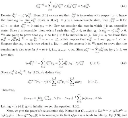
(a) For any state j≥k，we have

where qkk=1，and for j＞k，qkj=0 if j is a non-accessible state，i.e.=0 for all l∈N*，while qkj∈(0，∞) is the solution of the recurrence relation

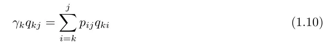
if j is an accessible state，i.e.＞0 for some l∈N*.

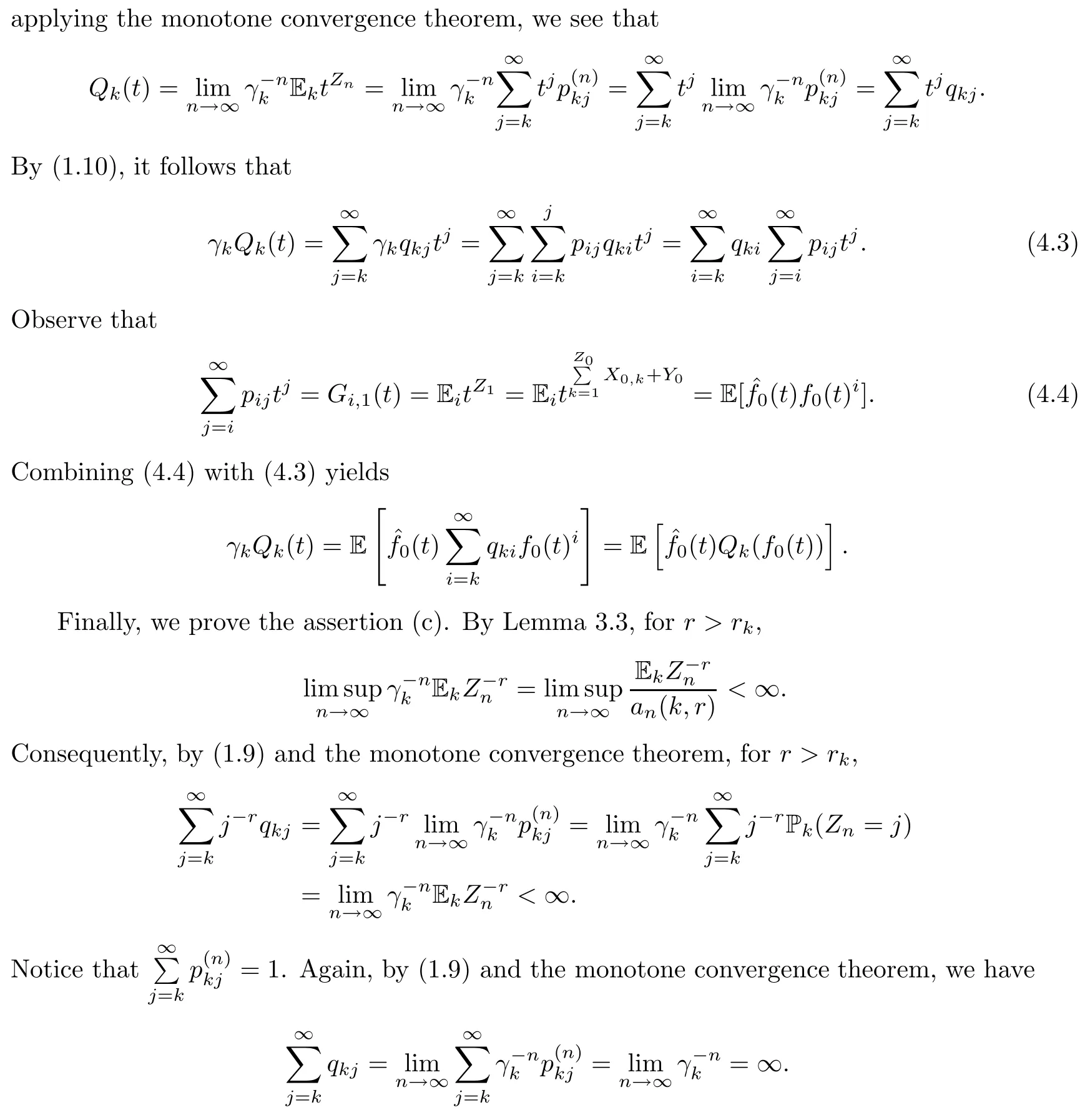
(b) Let Gk，n(t)=be the probability generating function of Znunder the probability Pk.For all t∈[0，1)，

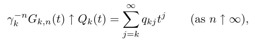
and Qk(t) satisfies the functional equation

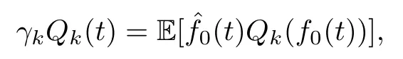
where f0(t)=andare the probability generating functions of X0and Y0，respectively，under the probability Pξ.

(c) Under the assumptions (H1) and (H2)，for any r＞rk，we have the series＜∞.In particular，the radius of convergence of the power series Qk(t) equals 1.

Theorem 1.2 is a generalizationof[19，Theorem 2.3]for BPRE.Since there is no immigration in BPRE，we have h0=1 and γk=.Similar aspects of BPRE were also studied in[5，8].For the case of a deterministic environment，similar results were shown in[28，35].

Corollary 1.3Assume (H0).If γk＞0，then for j≥k，

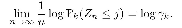
Corollary 1.3 is about the probability of staying bounded without extinction，which describes the asymptotic behaviour of Pk(Zn≤j) for BPIRE.For BPRE，Bansaye introduced the decay rate of Pk(Zn≤j) and gave an interpretation in a trajectory for the associated rare event{Zn=j}in[8];Grama et al.improved this result in[17].

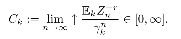
Theorem 1.2 can also be used to study the large deviations of Zn+1/Zn.This subject has attracted much interest;see for example[1，13，18，20，28，31，35].In particular，for classical Galton-Watson process，Athreya[1]showed that if p1mr＞1 and E (X0+Y0)2r+δ＜∞for some r≥1 and δ＞0，then

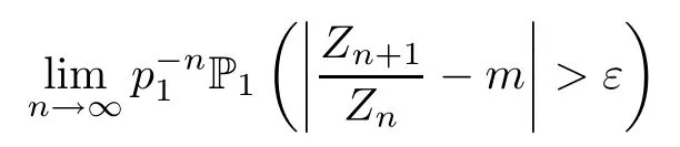
exists in[0，∞)，where m=EX0.Liu and Zhang[28]generalized such a result to a branching process with immigration，with p1replaced by h0.For BPIRE，an associated result is established by applying Theorem 1.2 as follows:

Corollary 1.4Assume (H0)，(H1) and (H2).If＜∞and＜∞for some r＞rk，then for every ε＞0，there exists Ck(ε)∈[0，∞) such that

For the case in a deterministic environment，since γ1=h0p1＜min{h0，p1}for the case k=1，Corollary 1.4 is actually a generalization and improvement of the results in[1，28].

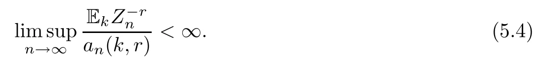
In order to further obtain some results similar to those that were shown in[18，31，35]on the large deviations of Zn+1/Zn，we need to find an equivalence to describe the convergence rates of the annealed harmonic moments of Zn.On this subject，readers can refer to[31]for the classical Galton-Watson process，[35]for the branching process with immigration，and[18]for BPRE.In term of research methods，in[31，35]，the authors divided the momentsinto three parts of integrals and then calculated the rates of each part by distinguishing three different cases according to the values of r.However，when the influence of the environment is taken into account，that classical method is no longer effective.For BPRE，a method of using a recurrence relation was adopted in[18].Following such an idea，we obtain the theorem below which describes precisely the decay rates of the harmonic moments.

Recall that in the de finition (1.8)，and rkis the solution of the equation γk=.For n∈N，set

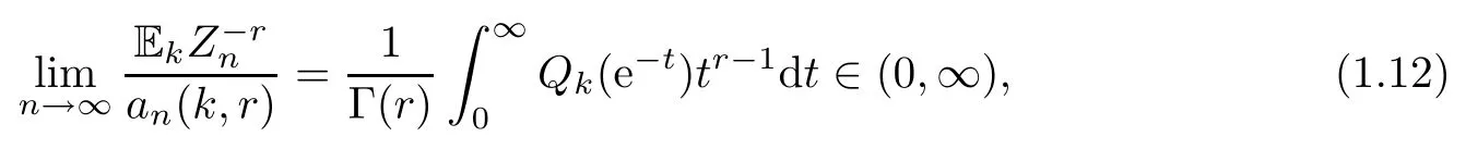
Theorem 1.5(Harmonic moments) Assume (H0)，(H1) and (H2).Then，

(a) For r＞rk，

(b) If Elog+Y0＜∞，for r≤rk，

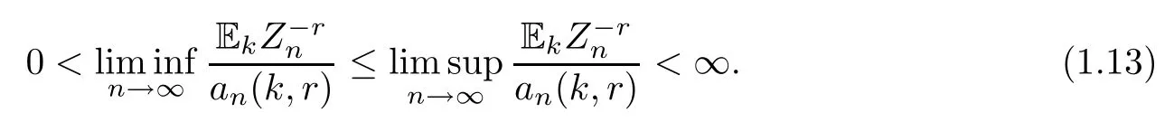
Theorem 1.5 gives a complete description of the asymptotic behaviour of the harmonic momentsof BPIRE.For BPRE，Grama et al.showed that=C (k，r)∈(0，∞) for all r＞0，where γk=(see[18，Theorem 2.1]).When r＞rk，Theorem 1.5(a) coincides with the result of[18]，but when r≤rk，instead of finding the precise limit as in[18]，we just obtain (1.13) in Theorem 1.5(b)，which also implies that the equivalent decay rate ofis an(k，r).In contrast with the result for BPRE，one should notice that for BPIRE，γk=becomes smaller，and hence rkbecomes larger.

Using Theorem 1.5，we can get the decay rate of the probability Pk(Zn≤kn)，where knis larger than k and may tend to infinity with a rate slower than the exponential rate eθn(θ＞0).For BPRE，corresponding results can be found in[7，18].

Corollary 1.6Assume (H0)，(H1) and (H2).Let (kn) be a sequence of positive numbers satisfying≥k andlogkn=0.If γk＞0，then

To prove Corollary 1.6，one just needs to notice that for n large enough (such that k≤kn) and r＞rk，Markov’s inequality yields

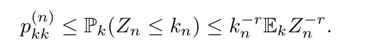
Applying Theorem 1.2(a) and Theorem 1.5(a)，we can obtain the conclusion.In particular，applying Corollary 1.6 with kn=j≥k leads tologPk(Zn≤j)=logγk，which means that the conclusion of Corollary 1.3 can also be deduced from Corollary 1.6.It is obvious，however，that the conditions of Corollary 1.3 are less than those of Corollary 1.6.If kntends to infinity with an exponential rate eθn(θ＞0)，we cannot reach (1.14) from Corollary 1.6.In this instance，one can expect thatlogPk(Zn≤kn)＞logγkif the limit exists.

Finally，we consider large deviations of logZn.Later we will particularly work on the lower and upper deviations Pk(Zn≤eθn) and Pk(Zn≥eθn) for θ＞0.Let Λ(t)=(t∈R) and Λ*(x)=(x∈R) be its Fenchel-Legendre transform.It is clear that

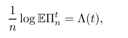
which implies that logΠnsatisfies a large deviation principle with the rate function Λ*(x)，according to the classical large deviation theory.As logZn=logΠn+logWn，it is possible that logZnsatisfies the same large deviation principle as logΠnin the case where Wnconverges to a non-degenerate limit W.Let

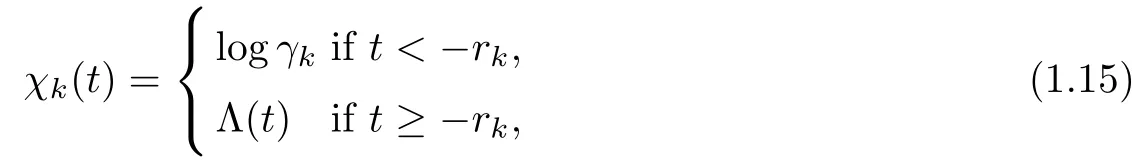
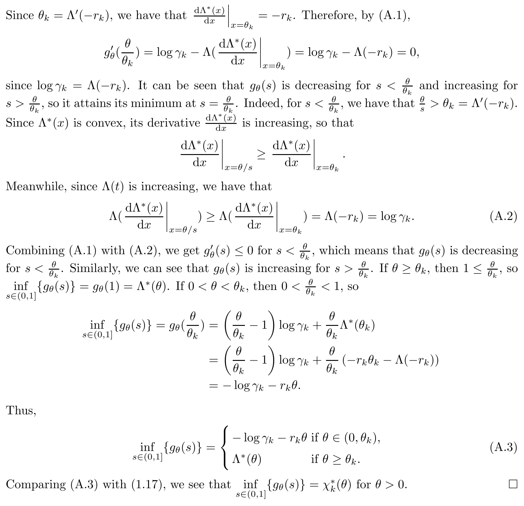
Since p0=0 a.s.，it is clear that χk(t)≥Λ(t)，so that≤Λ*(x).Denote θk=Λ′(-rk)，where Λ′(t)=is the derivative of the function Λ(t).We can calculate that

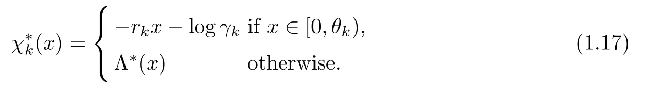
The graphs of the functionsand Λ*(x) are shown in Figure 1.

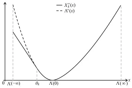
Figure 1 Graphs of the functions and Λ*(x)

In particular，if γk=0(i.e.，rk=∞)，we have χk(t)=Λ(t) and=Λ*(x).Noticing (1.16) and applying the Gärtner-Ellis theorem[10，p.53，Exercise 2.3.20]，we immediately obtain the following large deviation principle for logZn:

Theorem 1.7(Large deviation principle) Assume (H0)，(H1) and (H2).If γk=0，＜∞and＜∞for all p＞1，then for any measurable subset B of R，we have

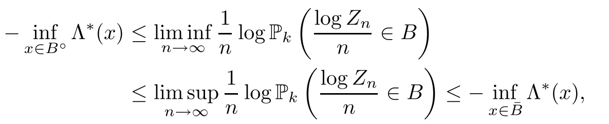
where B◦denotes the interior of B，andits closure.

The large deviation principle of logZnfor BPRE was proved by Huang and Liu in[21].Wang and Liu then extended that result to BPIRE[38，Theorem 7.2].Theorem 1.7 improves the condition of[38，Theorem 7.2].

Remark 1.1The conclusion of Theorem 1.7 was also shown in[37，Theorem 7.2]under the condition that p1=0 a.s..Here we relax that condition to γk=0.It is clear that γk=0 means that p1=0 or h0=0 a.s..We remark that[38，Theorem 7.2]was proved by using the harmonic moments of W of BPRE[16，Theorem 2.1].In[17]，the authors claimed that the assumptions (H1) and (H2) could be weakened.However，their proof was not correct，hence，in order to ensure[37，Theorem 7.2]，the assumptions (H1) and (H2) have still been necessary up until now.However，as we have pointed out before，the assumptions (H1) and (H2) can be replaced by the statement (1.6).

Under the conditions of Theorem 1.7，applying Theorem 1.7(by taking B=[θ，∞) and B=(-∞，θ]，respectively)，we can deduce the following results about the upper and lower deviations of logZn:

However，the conditions of Theorem 1.7 seem a little strong for investigating the upper and lower deviations of logZn.For example，Theorem 1.7 requires the existence of the positive momentsandfor all p＞1，but in general，in the case that the momentsandare finite for some p＞1，it still can be expected that the upper deviations of logZnfor certain θ(but not for all θ＞Elogm0) will be obtained.That is why，below，we investigate the upper and lower large deviations of logZnseparately without using Theorem 1.7.

Theorem 1.8(Large deviations) Assume (H0).Then，

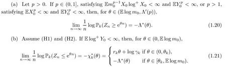
Compared with (1.18) and (1.19)，under weaker moment conditions and considering the case where γk=0 is possible，Theorem 1.8(a) reveals the upper deviations of logZnfor certain θ，and Theorem 1.8(b) shows the lower deviations of logZnfor all θ∈(0，Elogm0) with the rate functioninstead of Λ*.For BPRE，more precise properties about the upper and lower deviations of logZnwere shown in[5-7，18].

Remark 1.2If＜∞and＜∞for all p＞1，it can be seen that (1.20) holds for all θ＞Elogm0;i.e.，(1.18) holds.Indeed，by Theorem 1.8(a)，(1.20) holds for θ∈(Elogm0，Λ′(∞)).For θ≥Λ′(∞)，we have that Λ*(θ)=∞.By Markov’s inequality and Theorem 1.1，we have

which means that (1.20) also holds for θ≥Λ′(∞).For lower deviations，noticing that Pk(Zn≤eθn)=0 for θ≤0 and Λ′(-∞)≥0 under the condition (H0)，we have

for θ≤0.As there is no practical sense，we do not care about the case in which θ≤0.In particular，if γk=0，then=Λ*(θ)，so under the conditions of Theorem 1.8(b)，we see that (1.19) holds in the case γk=0.

2 Proof of Theorem 1.1

We introduce a change of measure.Denote the distribution of ξ0by τ0.Fix t∈R and de fine a new distributionas

where m (x)=E[X0|ξ0=x]=.Consider the new BPIRE whose environment distribution is τ(t)=instead of τ=.The corresponding probability and expectation are denoted by P(t)=Pξ⊗τ(t)，and E(t)，respectively.

To prove Theorem 1.1，we need a decomposition of the family tree.Assume that the whole family tree begins with initial ancestor particle k of generation 0，denoted by Ø1，···，Øk.For i∈{1，2，···，k}，the ancestor particle Øiproducesnumber of progeny particles of generation 1，denoted by Øi1，Øi2，···，，where=X0，i.At the same time，Y0immigrants join the family，denoted by 001，002，···，00Y0.All the new born particles and all the new immigrants form the first generation of the family.In general，the i-th particle of generation n，say u，produces Nuoffspring of generation n+1，denoted by u1，u2，···，uNu，where Nu=Xn，i;the new immigrants of generation n+1 are denoted by 0n1，0n2，···，0nYn.For a particle u，we denote bythe number of the n-th generation descendants originating from u.Let T be the shift operator that Tnξ=(ξn，ξn+1，···) if ξ=(ξ0，ξ1，···).If the environment is ξ and the particle u is of generation l，it is clear that the processforms a BPRE originating from a single initial particle with the random environment Tlξ，and.According to different origins，the population Zncan be decomposed as

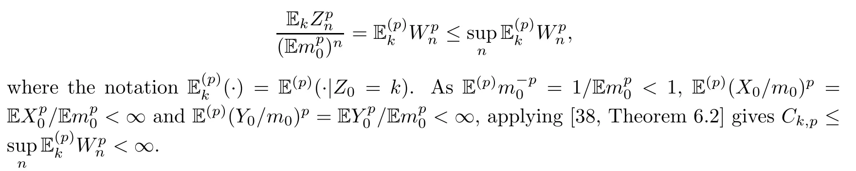
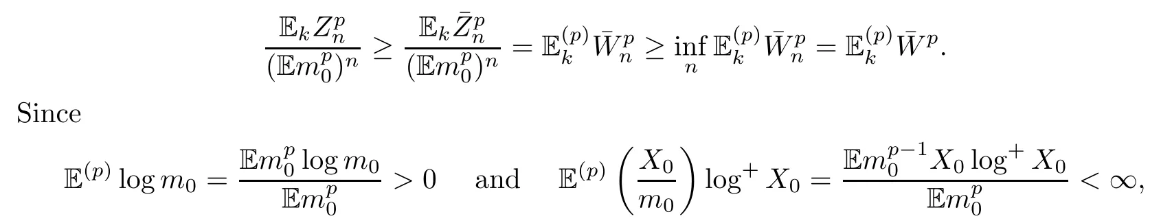
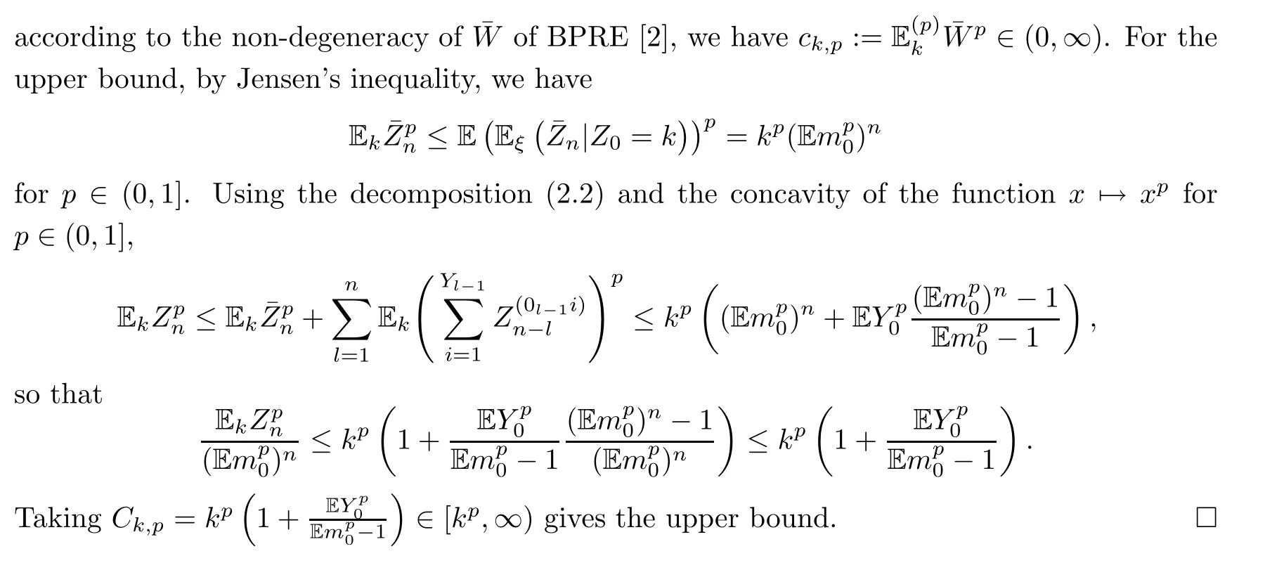
Proof of Theorem 1.1For the assertion (a)，since p＞1，notice that by (1.1) and by Jensen’s inequality，

which implies that Ck，p≥kp.On the other hand，using the change of measure，we see that

Now we consider the assertion (b).For the lower bound，we have

3 Upper Bound for Harmonic Moments

In this section，we shall show an upper bound for harmonic momentsfor r＞0，which is useful for the proofs of Theorems 1.2 to 1.8.

Lemma 3.1Let l≥1 be an integer.For different positive numbers α1，···，αl，set

in which s1，···，sl∈{0，1，2，···}.Then there exists C (α1，···，αl)∈(0，∞) such that

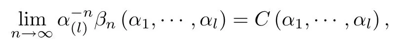
where α(l)=max{α1，···，αl}.

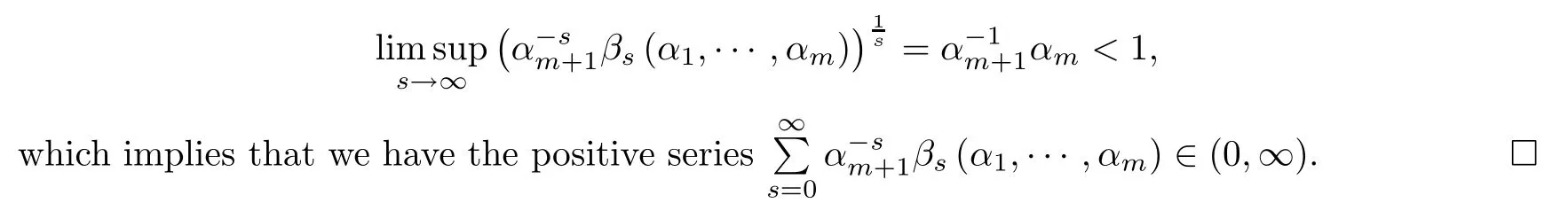
ProofWe will prove the conclusion by induction on l.The conclusion is clearly valid when l=1.Now supposing that the conclusion is true for l=m for some m≥1，we shall prove that the conclusion is still valid for l=m+1.Due to the inductive hypothesis，there exists C (α1，···，αm)∈(0，∞) such that

Without loss of generality，we can think that α1＜α2＜···＜αm+1.In this case，α(m+1)=αm+1.Notice that

We have

Thanks to (3.2)，we derive that

Following arguments similar to the proof of[20，Theorem 1.4](by considering k initial ancestors instead of one)，we can deduce the lemma below，which regards the critical value for the existence of the harmonic moments of the limitof BPRE originating from k initial ancestors.

Lemma 3.2Assume (H0)，(H1) and (H2).Let r＞0.Then＜∞if and only if＜1.

With the help of Lemmas 3.1 and 3.2，inspired by the method used in[17]，we obtain the following lemma，which reveals that=O (an(k，r)) as n tends to in finity:

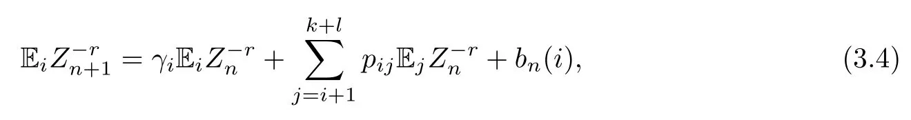
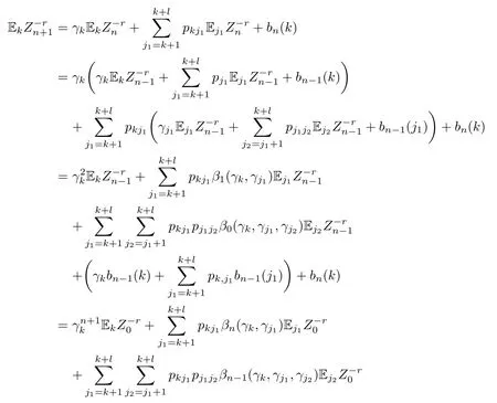
Lemma 3.3Assume (H0)，(H1) and (H2).If γk＞0，then

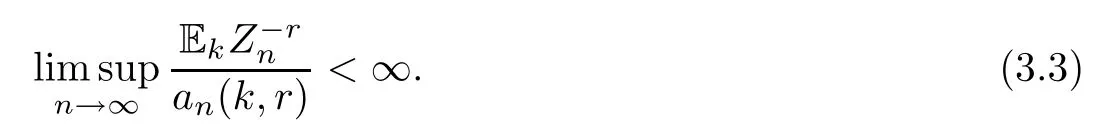
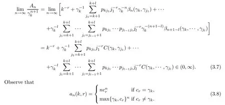
ProofFix k and r.Take an integer l≥0 large enough such that＜cr，and then fix this l.Set bn(i)=.By the Markov property，it can be seen that for every integer 0≤i≤k+l，

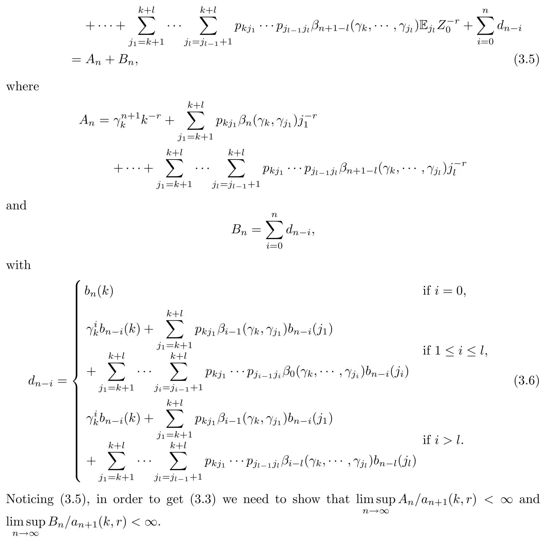
For An，noticing that the sequence (γk) is strictly decreasing，by Lemma 3.1 we obtain that

4 Proof of Theorem 1.2

Based on the upper bound offor r＞0(see Lemma 3.3)，in this section we give the proof of Theorem 1.2 and use Theorem 1.2 to prove Corollary 1.4.

Proof of Theorem 1.2We first give the proof of the assertion (a).By the total probability formula and the Markov property，for j≥k，

In other words，Qk(1)=∞，which means that the radius of convergence is ρ≤1.In order to prove ρ=1，we need to show that the series Qk(t) converges when|t|＜1.For|t|＜1，it is clear that|t|j≤j-rif j is large enough.Therefore，we know the convergence of Qk(t)=directly from the convergence of the series. □

Proof of Corollary 1.4Denoteand A (j，ε)=.Applying the total probability formula，we obtain that

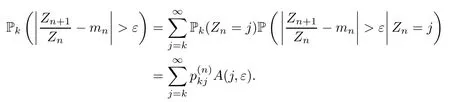
By the formula (1.9) in Theorem 1.2(a) and the monotone convergence theorem，we have that

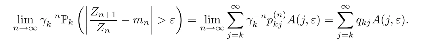
Set Ck(ε)=.We shall prove that there exists C (r，ε)∈(0，∞) such that A (j，ε)≤C (r，ε) j-rfor all j，which implies that Ck(ε)＜∞，by Theorem 1.2(c).It is easy to see that

For the first term on the right hand side of (4.5)，by Markov’s inequality，

For the second term on the right hand side of (4.5)，setting α=max{2r，r+1}，by Markov’s inequality again，we get that

By a consequence of the Marcinkiewicz-Zygmund inequality[29，Lemma 1.4]，

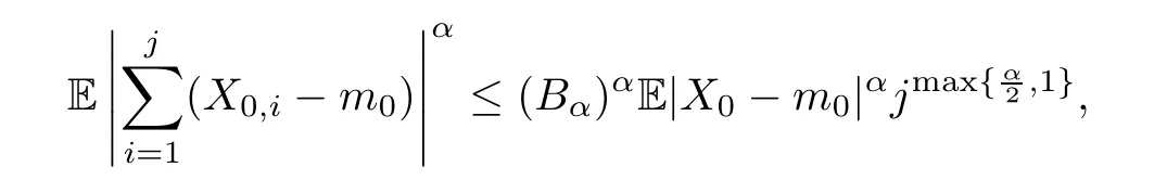
where Bα=2min{k1/2:k∈N，k≥α/2}is a constant depending only on α.Thus we have

Combining (4.6) and (4.7) with (4.5)，we see that A (j，ε)≤C (r，ε) j-rfor all j，where C (r，ε)=∈(0，∞). □

5 Proof of Theorem 1.5

In this section，we give the proof of Theorem 1.5.In Lemma 3.3，we have found an upper bound forfor r＞0.In order to obtain the lower bound，we need the non-degeneracy of the limit of the submartingale Wn.

Lemma 5.1Assume (H0).If Elog+Y0＜∞and EX0log+X0＜∞，then for any r＞0，under the probability P(-r)，Wnconverges a.s.to a limit W∈(0，∞)，so that＞0 for all k≥1 and s＞0.

ProofThe assumption (H0) implies that m0＞1 with positive probability，so we have that

Noticing (5.1) and that

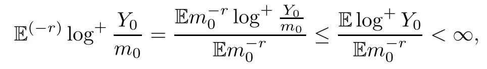
by[38，Theorem 3.2]we see that under the probability P(-r)，Wnconverges a.s.to a limit W∈[0，∞).In addition，noticing (5.1) and that

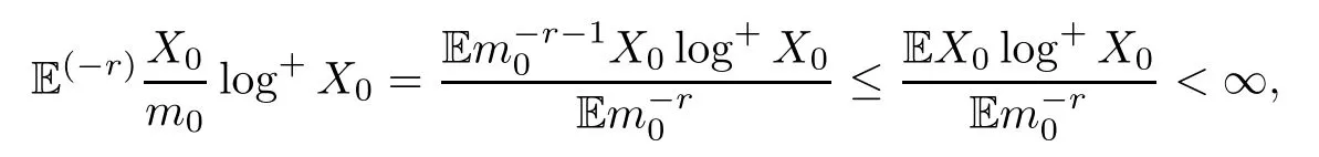
we deduce that under the probability P(-r)，＞0 a.s.according to the classic non-degenerate condition of BPRE (cf.[3]).As W≥，we have W＞0 a.s.The proof is complete. □

Proof of Theorem 1.5We first prove the assertion (a).For r＞rk，we have an(k，r)=.By the Markov property，we can get that，which means that the sequenceis increasing.Thus，we have the limit

By Theorem 1.2 and the monotone convergence theorem，

Meanwhile，we can calculate that

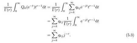
Combining (5.2) and (5.3) yields (1.12).

We next prove the assertion (b).Let us first consider the case where r=rk.We have that γk=crand an(k，r)=.By Lemma 3.3，we see that

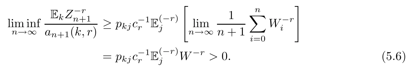
For the inferior limit，since=1 and pkk=γk∈(0，1)，there exists j＞k such that pkj＞0.By the Markov property，

Using (5.5)，and iterating，we obtain

Thus

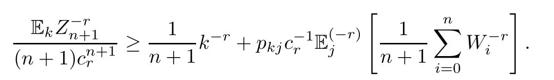
Combining (5.4) and (5.6) leads to (1.13) for r=rk.It remains to deal with the case where r＜rk.In this case，we have an(k，r)=.For the inferior limit of (1.13)，by Lemma 5.1 and Fatou’s lemma，we see that

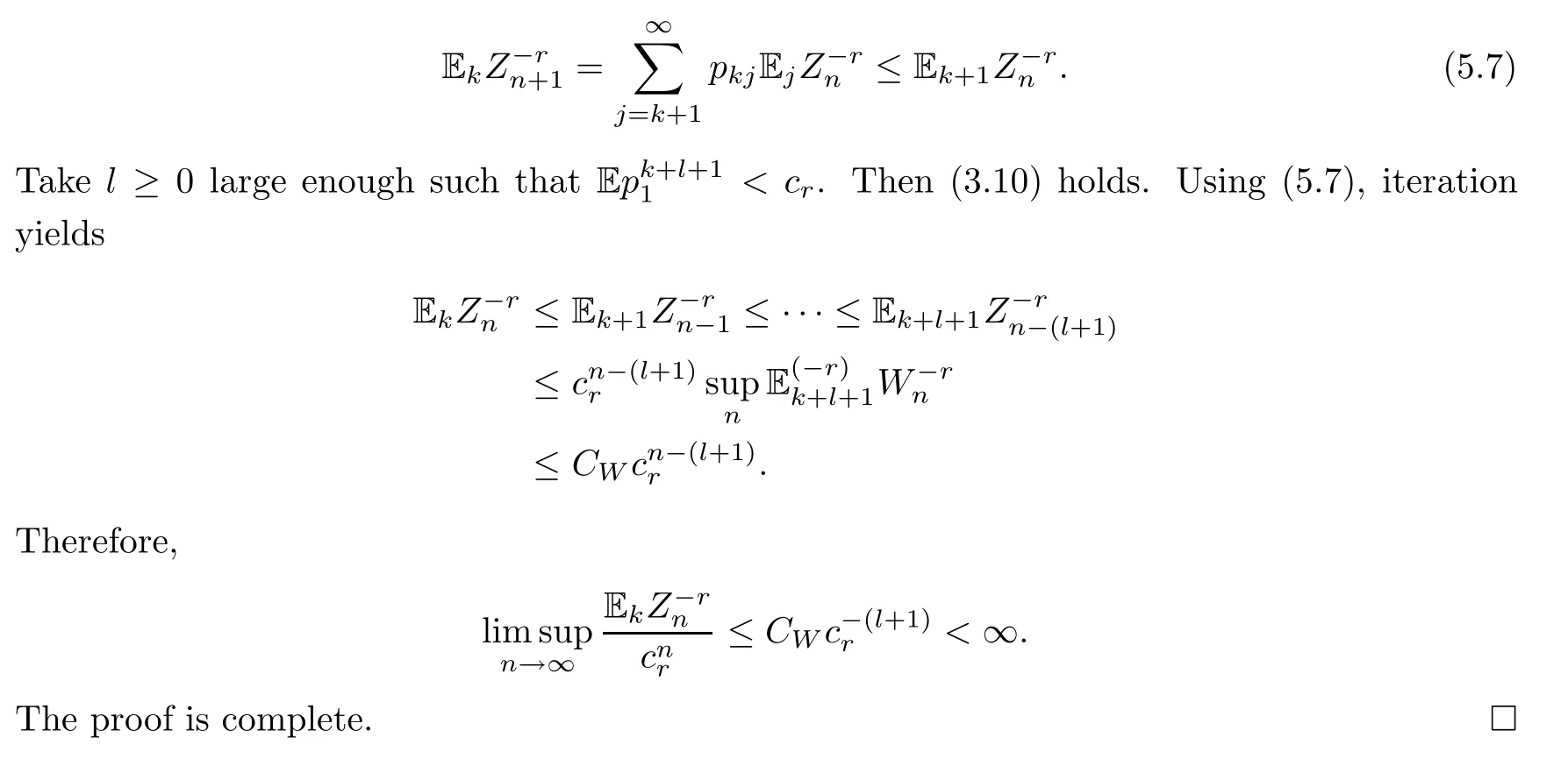
The superior limit of (1.13) we distinguish into two cases:(i)γk＞0;(ii)γk=0.For case (i)，the superior limit is given by Lemma 3.3.For case (ii)，we know from γk=0 that for any i，γi=0.By the Markov property，we have

6 Proof of Theorem 1.8

In this section，we focus on large deviations of logZn.For the lower deviations Pk(Zn≤eθn)，we will show upper and lower bounds，respectively，in the two propositions below.

Proposition 6.1Assume (H0)，(H1) and (H2).Then，for θ＜Elogm0，

ProofBy Markov’s inequality，for s＞0，

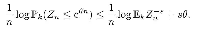
Letting n tend to infinity and using (1.16)，we get

Notice that (6.1) holds for all s＞0.Thus

We calculate that

Proposition 6.2Assume (H0) and (H1).If Elog+Y0＜∞，then，for θ＞0，

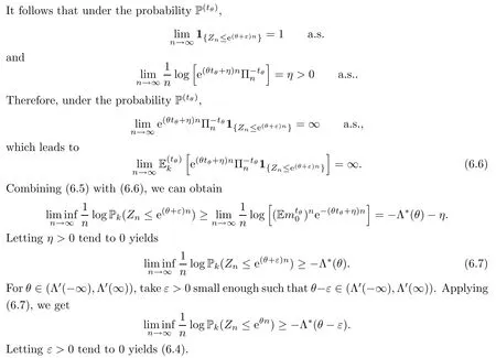
ProofWe first prove that for all θ，

Under (H0) and (H1)，the function Λ′(t) is continuous and increasing everywhere.If θ≤Λ′(-∞) or θ≥Λ′(∞)，then Λ*(θ)=∞and (6.4) holds naturally.Let θ∈(Λ′(-∞)，Λ′(∞)).Then there exists tθsuch that Λ′(tθ)=θ.With the help of the change of measure，for ε＞0 and η＞0，

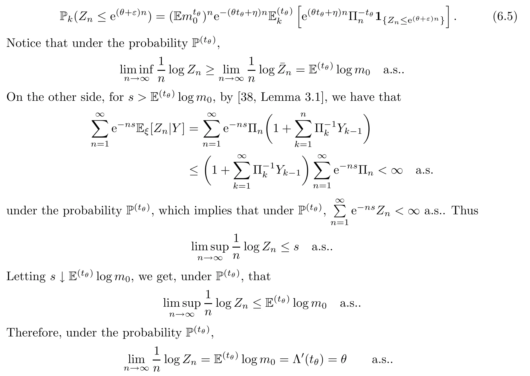
Now let us prove (6.3).If γk=0，then=Λ*(θ)，so (6.3) holds from (6.4).We next consider the case γk＞0.Taking t∈[0，1)，by the Markov property，we have

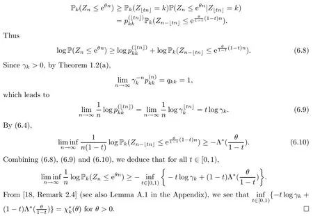
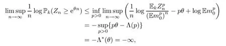
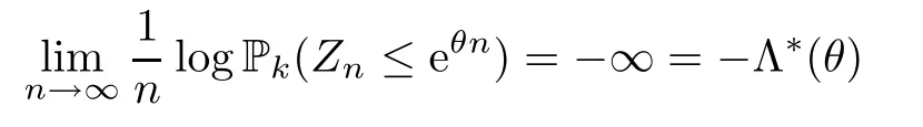
Proof of Theorem 1.8The assertion (a) is derived from Theorem 1.1 and[21，Lemma 3.1](see also[29，Theorem 6.1]).For the assertion (b)，the upper bound is from Proposition 6.1 and the lower bound is from Proposition 6.2. □

Appendix

In[18，Remark 2.4]，the authors pointed out thatfor θ∈(0，Elogm0).Here，for the reader’s convenience，we prove this result in a different way，by a method of direct calculations.

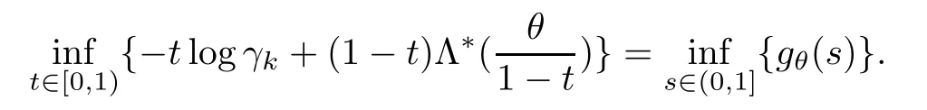
Lemma A.1Assume (H0) and (H1).For θ＞0，

ProofFor θ＞0，denote gθ(s)=(s-1) logγk+.By setting s=1-t，we see that

Noticing the fact that

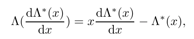
we calculate that