Ming-Wei Fang(方明卫), Jian-Chao He(何建超), Zhan-Chao Hu(胡战超), and Yun Bao(包芸)

School of Aeronautics and Astronautics,Sun Yat-sen University,Guangzhou 510275,China

Keywords: Rayleigh-B´enard,temperature fluctuation,distribution patterns,critical value

1. Introduction

Turbulent thermal convection occurs ubiquitously in both nature and engineering applications. Turbulent Rayleigh-B´enard convection(RBC),a closed fluid layer thermostatically heated from the bottom and cooled from the top, has chronically been used to study thermally-driven turbulence.[1-4]The enclosed working fluid forms convective motion through the buoyancy force produced by the temperature difference between the bottom and the top plates of a convection cell of heightH.

Turbulent RBC is controlled primarily by two dimensionless parameters, namely the Rayleigh number and the Prandtl number, defined asRa=αgΔθH3/(κυ) andPr=υ/κ, respectively, where Δθis the temperature difference,g=9.81 m/s2is the gravitational acceleration,andα,υ,andκare, respectively, the thermal expansion coefficient, the kinematic viscosity, and the thermal diffusivity. Apart fromH,the geometry of the convection cell also influences turbulent RBC. Therefore, in classical cubic and cylindrical cells, the aspect ratio also becomes a crucial parameter.

A core task in the study of turbulent RBC is to understand the heat transport in turbulent flows. In general, the Nusselt number,defined as

where〈···〉V,trepresents the average over space and time. It is usually calculated to reflect the strength of heat transport.In 2000, Grossmann and Lohse put forward the so-called GL theory[5-7]to predictNuaccording toRaandPrby decomposing the energy dissipation. There are two kinds of characteristic structures that are related to heat transport. One is the large-scale circulation, also known as ‘wind’ of the bulk fluid,[8-10]and the other kind of structure is a cluster of thermal plumes[11-13]that erupts intermittently from the thermal boundary layer. Previous researches have revealed that the heat transport is governed primarily by thermal plumes.[14-18]Moreover, the intensity of thermal plumes can be measured by the amplitude of local temperature fluctuations. In other words, the local temperature fluctuations and heat transport are closely linked to each other. According to the definition,the amplitude of local temperature fluctuations is measured at each specific point. To simplify the study, fortunately, it is convenient to examine the profile of the local temperature fluctuations,defined as

where〈···〉xrepresents the average over horizontal direction and the subscripttof time average is omitted. One can extract the information about flow state,plume distribution,and heat transport fromθrms(z). Therefore,θrms(z) has been studied frequently in previous work.

According to the Castainget al.’s theory,[19]Adrian identified two new profiles, termed asλ-I andλ-II models.[20]Recently,looking into the so-called mixing zone,the similarities inθrms(z)between the thin disk and the cylinder cells have been revealed.[21,22]He and Xia[23]investigatedθrms(z)in the shear-dominated zone and the plume-dominated mixing zone in a elongated cubic cell. They that the reportedθrms(z) is a power-law function ofzin the former region, and a logarithmic function in the latter region. Afterward,such a power-law has also been identified in non-elongated cells with different geometries.[24,25]There are also some experimental researches only focusing onθrmsin the cell center. TheRa-dependentθrmsshows the diverse traits in different geometries.[26-31]For example,Huang and Xia[32]discovered thatRa-scaling ofθrmsincreases with the aspect ratio.

In this paper, we present a direct numerical study on the characteristics ofθrms(z)in a two-dimensional(2D)turbulent RBC.Two different values ofPrare considered,i.e.,0.7 and 4.3. For both of them, the same range ofRais assigned:1×108≤Ra ≤1×1013. The rest of this paper is arranged as follows. In Section 2, we elaborate the governing equations and numerical methods. In Sections 3 and 4,characteristics of local temperature fluctuations and global temperature field forPr=4.3 andPr=0.7 are presented and discussed, respectively. TheRa-dependence of the mean temperature fluctuation is discussed in in Section 5. Our findings are summarized and also some conclusions are drawn in Section 6 finally.

2. Model and numerical methods

We perform direct numerical simulations (DNS) of 2D turbulent RBC in a square cavity. The non-dimensional governing equations under the Oberbeck-Boussinesq approximation are given by

whereu,θ,andpare respectively the non-dimensional velocity,temperature,and pressure,kis the vertical unit vector.RaandPrare the control parameters of the system as mentioned previously. Impermeable and no-slip boundary conditions are imposed on all walls. For temperature, the two vertical sidewalls are adiabatic, while the top and bottom plates are fixed atθt=-0.5 andθb=0.5,respectively. Thus,the dimensionless temperature difference between the two horizontal plates isΔ=θb-θt=1.Governing equations are solved by the parallel direct method(PDM)of DNS(or PDM-DNS)[33,34]with using staggered grids.

All simulations are carried out on the Tianhe-2 supercomputer.The parameters of all cases are summarized in Fig.1(a).Figure 1(b)presents a sketch of the time-averaged temperature fluctuation field, in which the thick black solid line (the central line)is the sampling region analyzed in this paper. In view of its symmetry, we choose the zone from the bottom to the center of the sampling region.

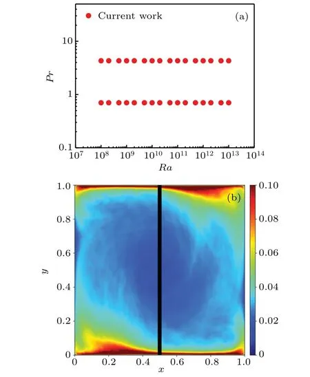
Fig. 1. (a) Simulated cases scattered in (Ra, Pr) plane. (b) Contour plot of time-averaged temperature fluctuation field,with solid line denoting sampling region.

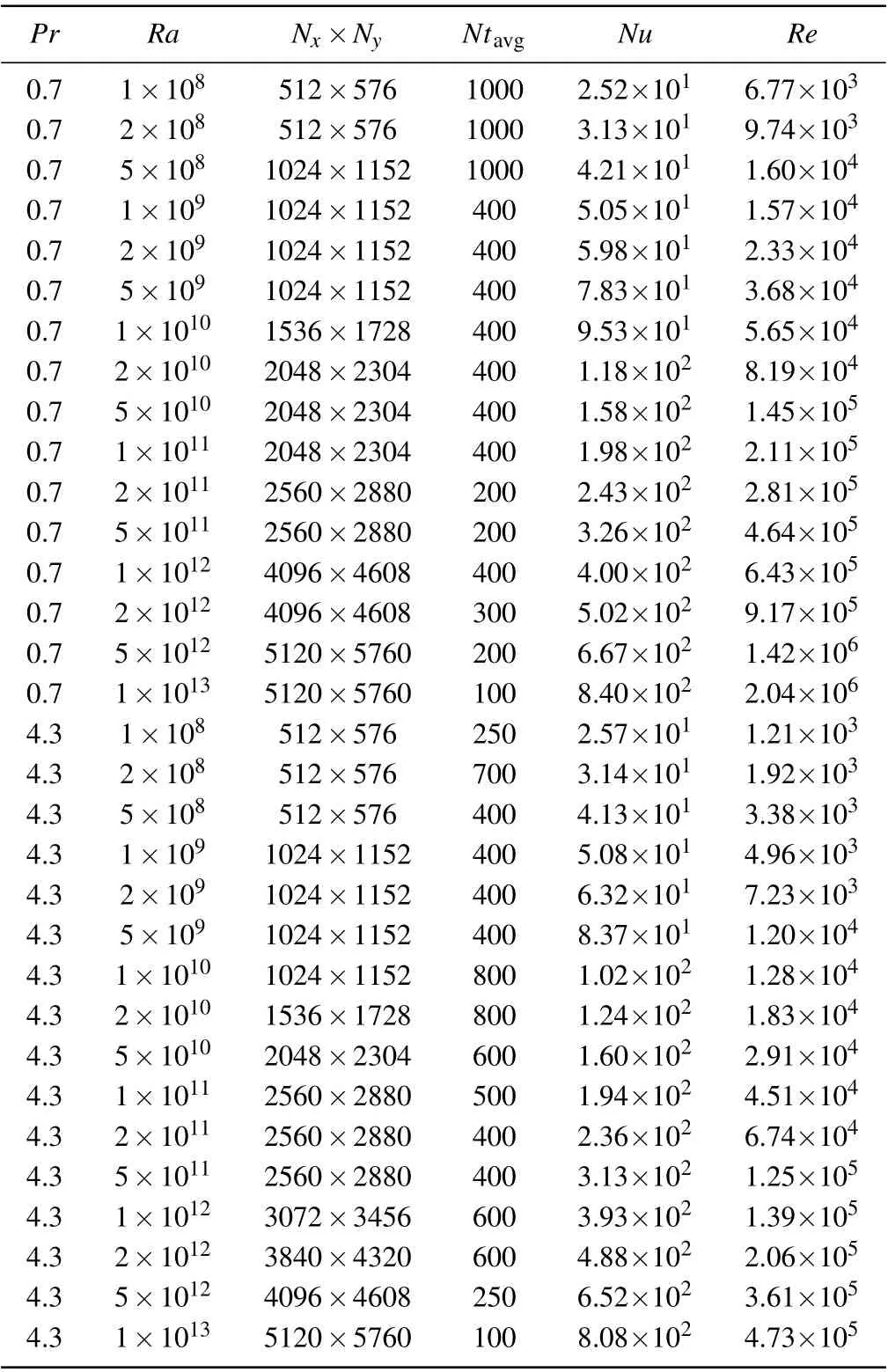
Table 1. Parameters of conducted DNS of 2D RBC.

Table 1 shows the detailed parameters of the simulation of RBC.The number of nodes in each direction of the computational mesh isNx×Ny·Ntavgis the number of dimensionless time (τ) units used for the statistical averaging.NuandRenumbers are the statistical non-dimensional heat transferNunumber and the small scale Reynolds number,respectively.

3. Results and discussion for Pr=4.3

3.1. Mean temperature proflie and probability density distribution of temperature

Fig.2. (a)Profiles of normalized mean temperature Θ at two different values of Ra for Pr=4.3. (b)Corresponding temperature fluctuation θrms profiles.

The thermal plumes,emitted intermittently from the conducting plates,play an important role in heat transfer of turbulent thermal convection. The plume is the only thermal structure in the system,and its temperature characteristics are analyzed through temperature statistics. We present the statistical results of temperature at different values ofRa.thermal BL. Whenz/δ>1, the mean temperature gradually approaches to the central temperature. AtRa=1×1011, it tends to the central temperature more slowly. After three thermal BLs,the temperature profiles overlap again and reach the core temperature. Note also from Fig. 2(b) that the temperature fluctuation profiles show significantly different characteristics. The temperature fluctuation rises fast and reaches a maximum value, then always decays forRa= 1×1011.While forRa=1×109, the temperature fluctuation change is relatively small. The overall temperature fluctuation first increases, then decreases, and finally rises slowly. The temperature fluctuation profiles of twoRanumbers reach their corresponding maximum values near the thermal boundary layers.

Fig.3. PDF of local temperature and normalized temperature fluctuations for several values of Ra.

Figure 2 shows the calculated mean temperature profileΘ(open circles) and temperature fluctuation profileθrms(solid circles) each as a function of normalized distancez/δfrom the lower plate along central axis region of flow space for two typicalRavalues, withPr= 4.3 fixed. Hereδis the thickness of the thermal boundary layer(BL)defined by the slope method.[35]The mean temperatureΘis normalized and defined asΘ=[θbot-〈θ(x,z)〉x]/θbot,whereθbotand〈···〉xare respectively the temperature of the bottom plate and the average over horizontal direction. In Fig. 2(a), the mean temperature profiles overlap each other and rise rapidly inside the

Temperature probability density distribution (PDF) represents the proportion of the temperature distribution in the region,where PDF stands for probability density distribution.Figure 3(a) shows PDF of the temperature in the central axis region (from the bottom to the center) for different values ofRa. It is seen that the PDFs from five different values ofRaare very similar,and can be well described as exponential functions. The bulk temperature s skews significantly towards higher temperature. It is seen that asRaincreases, the probability of occurrence of lower temperature at the left tail decreases,while the phenomenon does not exist for higher temperature at the right tail. By measuring the temperatures of six different positions on the central axis,Zhou and Xia[35]found that the PDF of temperature in the boundary layer presents a nearly Gaussian shape, and the PDFs of other positions are different from each other.

Figure 3(b)shows the plots of the corresponding PDFs of the normalized temperature fluctuations obtained at different values ofRa. It is seen that all the PDFs exhibit almost an exponential shape of symmetry. While,in previous experiments it was found that the normalized temperature fluctuation in the center of the cell can be well described by a stretched exponential function.[31,32,36,37]The right tail shifts slightly downward highRa, indicating that the probability of larger temperature fluctuation decreases. The PDF form of temperature fluctuation has apparent distinctions for different flowing states.

3.2. Local temperature fluctuations

Plume, as the most prominent thermal structure in RB system,is closely related to the temperature fluctuation of the system, and it possesses its own characteristics and motion mode. The local temperature fluctuation is an important indication for plume spatial distribution. Figure 4 shows a loglog plot of temperature fluctuationθrmsas a function of the normalized distancez/δfor various values ofRa.

Fig. 4. Profiles of measured temperature fluctuation θrms corresponding to half the black solid line region in Fig.1(b)(from bottom plate to center),and at various values of Ra from 1.0×108 to 1.0×1013.

Figure 2 shows that the temperature fluctuation profile increases linearly in the boundary layer, and then decays away from the plate. It can be seen from Fig. 4 that there are two distribution patterns. Under 1×108≤Ra ≤5×109, the temperature fluctuation profiles have two peaks at aboutz/δ=1 andz/δ= 10 respectively. The two peaks of the temperature fluctuation profiles decrease withRaincreasing. It is seen from this figure that forRagreater than 5×109, the temperature fluctuation profiles all collapse into a single curve. Theθrmsprofiles rise first and then decrease when leaving from the bottom plate,reaching a peak at aboutz/δ=1.

The comparison between the two types ofθrmsprofiles ofRa ≤5×109andRa ≥1×1010shows that theθrmsprofiles are overall significantly larger forRa ≥1×1010. This means that system flow status and plume distribution are obviously different.

Figure 5 shows the plots of the normalized temperature fluctuationθrms/θrms,maxversus z/δand in these figures the values ofθrmswere measured in the thin disk from Wanget al.[21,22]and in the cylinder from Wanget al.,[22]respectively,whereθrms,maxrepresents the maximum value ofθrms.It shows clearly that all profiles of the normalized temperature fluctuationθrms/θrms,maxfor different values ofRacollapse into a single curve quite well inside the thermal BL, which implies that in theθrms/θrms,maxprofiles there exists a self-similarity or independence ofRa. Beyond the boundary layer,for different values ofRa,θrms/θrms,maxprofiles take on different distribution characteristics. In the range ofRa<1×1010, when moving away from the BL, temperature fluctuation profilesθrms/θrms,maxdecrease withz/δincreasing, then moderately increase in the region 1≤z/δ ≤10,and finally drop dramatically. Withz/δvarying from 1 to 10, the ascending slope gradually decreases withRaincreasing. The appearance may be caused by corner rolls’ motion. ForRa ≥1×1010, theθrms/θrms,maxprofiles always decrease with increasing the distance from the BL.As shown in Fig.5,our DNS results accord well with the experimental data measured by Wang (red and blue open circles)in the range ofz/δfrom 1 to 8 and the DNS results obtained by Wang(green solid circles)for 1≤z/δ ≤2.

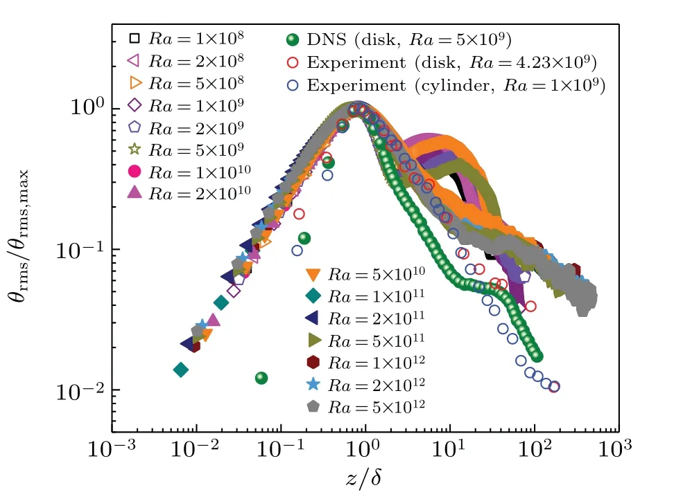
Fig. 5. Here data the same as in Fig. 4 but normalized by maximal value θrms,max of temperature fluctuations θrms where green solid circles and blue empty circles are for thin disk and cylinder, taken from Ref. [21] and red open circles for thin disk taken from Refs.[21,22].

Note that outside 10 BLs,the profiles of theθrms/θrms,maxpresented expose some different features from the results acquired Wang, where the temperature fluctuation is found to decrease continuously,probably due to the fact that the effect of corner rolls for their experiments conducted in the thin disk is neglected.However,inside the thermal BL,our data slightly deviate from the experiment data,which may be because there are too few data measured in the boundary layer.

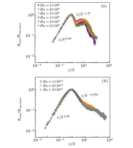
Fig.6. Here data the same as those in Fig.5,but divided into two plots: (a)from 1.0×108 to 5.0×109, (b) from 1.0×1010 to 5.0×1012, where solid lines show the power-law fits.

To show the temperature fluctuation profiles more clearly,in the following Fig.6,we plot the same data as those in Fig.5 but two forms drawn separately corresponding to different values ofRa.

Figure 6(a) presents the normalized temperature fluctuation profilesθrms/θrms,maxin the range ofRafrom 1×108to 5×109. It is seen that the temperature fluctuationθrms/θrms,maxremains unchanged withRavarying and scales withz/δin boundary layer, which is in excellent agreement with the previous experimental results.[22,26]The temperature fluctuationθrms/θrms,maxcan be well described by the power law,θrms/θrms,max～(z/δ)0.99withz/δ ≤1, andθrms/θrms,max～(z/δ)-1.27in the region 1≤z/δ ≤2.

It is seen from Fig. 6(b) that in a wide range ofRa,i.e.,Ra ≥1×1010and these profiles collapse into a single curve irrespective ofRa, but there is slight fluctuation in the mixing zone 6≤z/δ ≤50. In the boundary layer, the solid line represents a best fit to the data:θrms/θrms,max～(z/δ)0.99,this scaling law is the same as the one in Fig. 5(a). In the region 1≤z/δ ≤5, the data can be well described by a power law,i.e.,θrms/θrms,max～(z/δ)-0.978that are consistent with the DNS result[22]for the thin disk.

3.3. Global flow features

Regarding the two different characteristics of the temperature fluctuation profiles discussed above,to find the real variation characteristic for the temperature fluctuation, now we come to discuss the temperature and flow characteristics of the system in detail by visualizing the instantaneous temperature fields.

Figure 7 shows the typical example of instantaneous temperature fields atPr=4.3 with five different values ofRa,in which the colormap limit for all temperature snapshots in our study is set between-0.1≤θ ≤0.1,so that the flow structure can be shown clearly. As shown in Figs. 7(a) and 7(b), the overall flow pattern consists of a large clockwise titled-ellipse motion (large-scale circulation) and two corner rolls diagonally opposite to each other. This flow pattern is the same as those observed in previous studies.[38,39]WhenRaincreases toRa=1×1010(Fig.7(c)),surprisingly,the LSC and two secondary rolls vanish,and the whole flow becomes chaotic. AsRafurther increases,it is clearly seen from Figs.7(d)and 7(e)that the flow becomes more chaotic and there are a lot of free cold and hot small vortices. We note that the instantaneous temperature fields before and afterRa=1×1010show completely different flow states, suggesting that the mechanism of temperature fluctuation distribution showing two different characteristics may be due to the convective flow change.

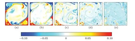
Fig.7. Typical evolution of the instantaneous temperature field with Ra at Pr=4.3: (a)Ra=1×108,(b)Ra=1×109,(c)Ra=1×1010,(d)Ra=1×1011,(e)Ra=1×1012.

4. Results and discussion for Pr=0.7

The temperature fluctuation and flow structure are discussed in detail forPr=4.3 above. Next, we will study the temperature fluctuation and flow characteristics withPr=0.7.

Figure 8(a) shows the variations of temperature fluctuationθrmswith distancez/δfrom the bottom plate for different values ofRaand fixedPr=0.7. It is seen that the temperature fluctuationθrmsprofiles also present two different morphologies. To compare withPr=4.3,we note that the turning point of theRaof the two morphologies becomesRa=1×109and the temperature fluctuationθrmsdoes not rise outside the BL.We plot, in Fig. 8(b), the same data as in Fig. 8(a) butθrmsnormalized by maximal valueθrms,max. Inside the BL,all data profiles for different values ofRaalways collapse on the top of each other. The solid line represents a power-law fit to the data,θrms/θrms,max～(z/δ)0.98. For 230 forRa ≥1×109.

Figure 9 shows snapshots of the typical temperature field at five different values ofRaforPr=0.7. It is seen from Fig. 9(a) that the flow consists of large-scale circulation of an ellipse in the bulk and two corner rolls in the upper left and lower right corners. WhenRaincreases toRa=1×109,the flow structure becomes unexpectedly different, the largescale circulation of ellipse and two corner rolls disappearing,the convection flows disorderly. Comparing with diverse characteristic of the temperature fluctuation profiles observed in Fig.8,we find the flow status transitionRais consistent with the turning point of fluctuation profiles morphology.

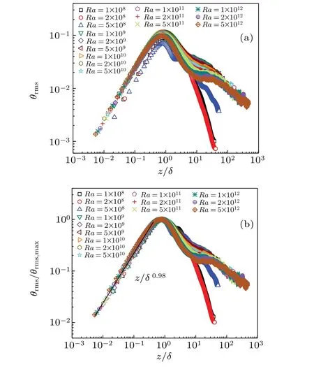
Fig.8. (a)Profiles of temperature fluctuation θrms for different values of Ra,and(b)normalized θrms/θrms,max profiles.

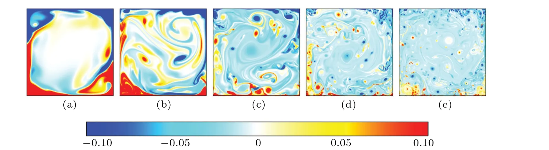
Fig.9. Typical evolution of instantaneous temperature field with Ra at Pr=0.7: (a)Ra=1×108, (b)Ra=1×109, (c)Ra=1×1010, (d)Ra=1×1011,(e)Ra=1×1012.

The different distribution characteristics of the temperature fluctuation correspond to various flow statuses and plumes’ morphologies, and the physical mechanism of the phenomenon correlation will be further discussed.

5. The Ra dependence of temperature fluctuation properties

Finally,we discuss theRadependence of〈θrms〉Vfor the temperature fluctuation atPr=0.7 and 4.3,respectively. Here〈···〉Vrepresents a time average and a spatial average in the black shaded region in Fig.1(b)(from the bottom plate to the center). Figure 10 show a log-log plot of the temperature fluctuation〈θrms〉Vas a function ofRa.

It is seen from Fig. 10(a) that the〈θrms〉V versus Rahas an apparent transition atRa=1×109. WhenRais below this transition point,there is no obvious characteristic law that describes the relation of〈θrms〉VwithRa. At the transition point,〈θrms〉Vsuddenly increases, then decreases asRaincreases and the change relation between the two quantities is described as〈θrms〉V～Ra-0.15±0.01. Note that the scaling exponent reported here accords well with the previous measurement conducted by Zhou and Xia[35]in a rectangular cell.

Figure 10(b) shows the〈θrms〉Vas a function ofRaatPr=4.3. It can be seen that a similar transition point also exists, which is obviously larger than that atPr=0.7, i.e.,Ra= 1×1010. Below the transition point,〈θrms〉Vexhibits reduction along with obvious fluctuations. WhenRais beyond this transition point,〈θrms〉Valso decreases withRaincreasing and the data can be well described by the power law,〈θrms〉V～(-0.68±0.01)Ra-0.14±0.01. Interestingly, the exponent of the power law is the same as the results obtained from experiments.[19,26,31,37]

Fig. 10. Variations of 〈θrms〉V versus Ra in central axis range of cell: (a)Pr=0.7,(b)Pr=4.3. The solid lines are power-law fits.

6. Conclusions

In this work,we systematically study the statistical properties of the local temperature fluctuation in 2D RBC of aspect ratio unity with the Prandtl number fixed at 0.7 and 4.3 and the Rayleigh number varying from 1×108to 1×1013. For the study of temperature fluctuation in the central axis region,we summarize the major findings as follows.

(i)The PDF of the temperature and the temperature fluctuation generally presents a consistent form and can be well described by an exponential function at fixed Prandtl number 4.3 for different values ofRa. Integrally,the temperature PDF skews significantly towards higher temperature. The PDF of the temperature fluctuation takes on a symmetrical exponential shape,nevertheless,on the whole it slightly inclines to the right atRa=1×1013. It is found that the PDF of the temperature and the temperature fluctuation have similar characteristics under eachRa.

(ii) With the variation ofRa, the profile of temperature fluctuation exhibits two different distribution characteristics atPr= 0.7 andPr= 4.3. WhenPr= 4.3, in the BL region, all the temperature fluctuation profilesθrmscollapse into a single master curve. Beyond the boundary layer,theθrmsprofiles decrease withz/δincreasing, then increase gradually and finally drop dramatically forRa< 1×1010.WhenRa>1×1010, theθrmsprofiles continuously decrease and overlap with each other. Normalized fluctuation profilesθrms/θrms,maxalso have similar features. Inside the BL,there is a power law,θrms/θrms,max～(z/δ)0.99. Outside the boundary layer, underRa ≤5×109, theθrms/θrms,maxcan be described by a power law,θrms/θrms,max～(z/δ)-1.27withz/δ ≤2. ForRa ≥1×1010,θrms/θrms,max～(z/δ)-0.978withz/δ ≤5. In particular,whenPr=0.7,the temperature fluctuationθrms/θrms,maxprofile distribution is similar to that whenPr=4.3. Especially,beyond the temperature boundary layer,the profile always drops and does not upraise. The two different distribution characteristics of temperature fluctuations are closely related to whether there are stable large-scale circulations and corner rolls in the instantaneous flow.

(iii) The〈θrms〉V, the spatiotemporal averages of local temperature fluctuation, have similar dependence onRafor two differentPrnumbers.ForPr=0.7,whenRais above this transition point,i.e.,Ra=1×109,〈θrms〉Vas a function ofRais well described by the power law〈θrms〉V～Ra-0.15±0.01.WhilePr= 4.3, the transition point is given byRa= 1×1010. Beyond this transition point, there is also a power law〈θrms〉V～Ra-0.14±0.01.

Acknowledgements

Project supported by the National Natural Science Foundation of China (Grant No. 11772362),the Shenzhen Fundamental Research Program (Grant No. JCYJ20190807160413162), and the Fundamental Research Funds for the Central Universities, Sun Yat-sen University,China(Grant No.19lgzd15).