Jintao Yang(杨锦涛) Junpeng Cao(曹俊鹏) and Wen-Li Yang(杨文力)

1Beijing National Laboratory for Condensed Matter Physics,Institute of Physics,Chinese Academy of Sciences,Beijing 100190,China

2School of Physical Sciences,University of Chinese Academy of Sciences,Beijing 100049,China

3Songshan Lake Materials Laboratory,Dongguan 523808,China

4Peng Huanwu Center for Fundamental Theory,Xi’an 710127,China

5Institute of Modern Physics,Northwest University,Xi’an 710127,China

6School of Physical Sciences,Northwest University,Xi’an 710127,China

7Shaanxi Key Laboratory for Theoretical Physics Frontiers,Xi’an 710127,China

Keywords: machine learning,quantum dynamics,open quantum system

1. Introduction

Machine learning is a very important technique in the study of modern physics, mathematics, chemistry, and medicine. Artificial neural network is a powerful tool to realize the machine learning. Focus on the physics, artificial neural networks are used to study phase transitions and critical phenomena.[1-13]topological nature of quantum states,[14-18]many-body correlated effects,[19-26]optimization of numerical simulations,[27-29]quantum error correction codes,[30-33]and so on.[34-37]

Recently, machine learning is also applied to the open quantum systems which have many applications in various fields such as solid state physics,quantum chemistry,quantum sensing, quantum information transport, and quantum computing. Luchnikovet al.applied the supervised learning to the open quantum system.[38]By constructing the likelihood function of a specific sequence of physical quantity and using it as a loss function for back-propagation, they simulated the model Hamiltonian of an open quantum system.

Neural network has been used in the machine leaning extensively. By adjusting the connection weights among neurons in the neural network, machine learning can be carried out. Later, the neurobiology experiments show that the static weights can also be used to realize the fast learning.[39]

In this paper, we study the non-Markovian dynamics of an open quantum system by constructing a biological recurrent neural network. With the help of stored data library, all the weights after appropriate pre-training are fixed. Thus the weights learning is not required and the dynamical properties can be learned quickly.[40]Then we generate the dynamical behaviors of physical quantities by this kind of supervised dynamical learning.

There are two ways to carry out the machine learning.One is simulating the system Hamiltonian. We show that only if the Hamiltonian is generated accurately, the corresponding dynamic behaviors can be true. The other is the dynamical learning of time evolution of the physical quantities. We find that the neural network with static weights can give the dynamic properties very well.

2. Non-Markovian quantum dynamics

Quantum dynamics is the result of interactions between the system and the environment.Generally,the environment is complicated and can affect the dynamical behavior of the system, thus can be regarded as an effective reservoir. From the dynamical properties of the system, some information about the environment could be obtained. The contributions of environment are mainly attributed to the memory effects accompanying non-Markovian dynamics.

When measuring a quantum system,if the degree of freedom of effective reservoir is equal to one, the system evolution is Markovian. That is to say, the measurement results at current moment are only related to the measurement values at previous moment. Thus the present results do not depend on the overall measurement results in the earlier period of time.

In this paper, we consider the non-Markovian quantum dynamics and the system is described as[38]

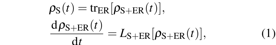
whereρS(t)is the density operator of the system,ρS+ER(t)is the density operator of system and environment,andLS+ERis the generator of non-Markovian process. In system (1), the environment is divided into two parts. The first part carries the memory and is responsible for non-Markov dynamics.The second part does not have the memory and leads to the Markovian dissipation and decoherence between the system and the effective reservoir.

Now,we carry out the machine learning. The density operatorρS(t)can not be achieved by the machine through a single learning. Only through many times of learning, the relevant information about the system can be obtained. The learning means the measurement, that is acting a projection operator on the system and the effective reservoir. Considering a series of projection measurements with different time, the measurement results seem useless,because the wave function of quantum system collapses with each measurement. However,such series of measurement results do contain some necessary information related with the system. It is proved that an enormous number of measurements has a pattern which can be recognized by the machine.[38]Then we can extract the effective information about the system from the corresponding pattern.

In order to learn the non-Markovian dynamics, we first need to construct a dataset for machine learning. We arrange the projection measurements in the order of time. In the process of obtaining training data,the time evolution rule is given by the generatorLS+ER.

The dynamical properties of the system are quantified by the time evolution operatorU(t)= e-iHt/¯h, whereHis the Hamiltonian. The time evolution of a state satisfies|ψ(t)〉=U(t)|ψ(0)〉,where|ψ(0)〉is the initial state. Then the density operator readsρS(t)=|ψ(t)〉〈ψ(t)|. We note that the time evolution operator can also generate the training dataset.

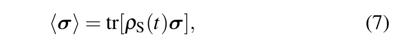
For simplicity,we choose the observable physical quantities as the expected values of Pauli matrices

and study their dynamical properties. It is clear that the expected values depend on the time evolution operator thus the Hamiltonian. Therefore, in order to obtain the dynamical properties of these physical quantities, we should learn the Hamiltonian first. Here we simulate the Hamiltonian by using the supervised learning. Obviously, the results are better when the simulated Hamiltonian is closer to the actual values.

3. Learning of Hamiltonian

In this section, we start from the Hamiltonian of a given quantum system to show the machine learning results.We randomly generate a Hamiltonian as

whereWis ad2×d2Hermitian matrix andIis thed×didentity matrix. Thus the Hamiltonian is ad3×d3matrix. For simplicity,we putd=2 and the matrix elements ofWtake the random complexes with the absolute values of both real and imaginary parts less than one. The Hamiltonian in Eq.(3)includes the system and the environment. The dimension of the system isd. The environment is divided into two parts and the dimension of each part isd. TheWin Eq.(3)corresponds to the combination of the system and the first part of the environment. The first part carries the memory and is responsible for the non-Markov dynamics. The second part does not have the memory and leads to the Markovian dissipation. For simplicity, we set the second part of the environment as the identity matrix.

We first learn the Hamiltonian(3)by using the supervised learning. The main idea of supervised learning is as follows.During the learning,we define a loss functionp({Ej}Nj=1|Hi),

whereEjis the projection operators acting on the system and the effective reservoir,Nis the total number of projectors with different time andHiis the current Hamiltonian. The set of projectors{Ej}Nj=1supplies the training set for the machine learning. The loss function is used to quantify the difference between the learned Hamiltonian and the real one. During the training, the learned Hamiltonian changes with each steps. The loss function can be increased as much as possible through the gradient ascent. When the log likelihood(1/N)logp({Ej}Nj=1|Hs) of the trained systemHsis equal to the actual value(1/N)logp({Ej}Nj=1|H)which is obtained by the given Hamiltonian(3),we expect that the learned HamiltonianHsequals to the real one(3)and the dynamical evolution of the physical quantities given byHsmeet the actual values.

The log likelihood of supervised learning result and the actual value are shown in Fig. 1(a). We see that after completing the training, the log likelihood of the trained systemHsequals that of the real system with the epochs steps larger than 75. Then we calculate the physical quantities〈σ〉and the results are shown in Figs. 1(b)-1(d). Here, the blue lines denote the supervised learning results while the red lines denote the actual values which are obtained form Eqs. (2) and(3). We find that the dynamical evolution of physical quantities obtained from the trained systemHsare slightly different from the actual values, although the log likelihood of trained system is the same as the actual value.

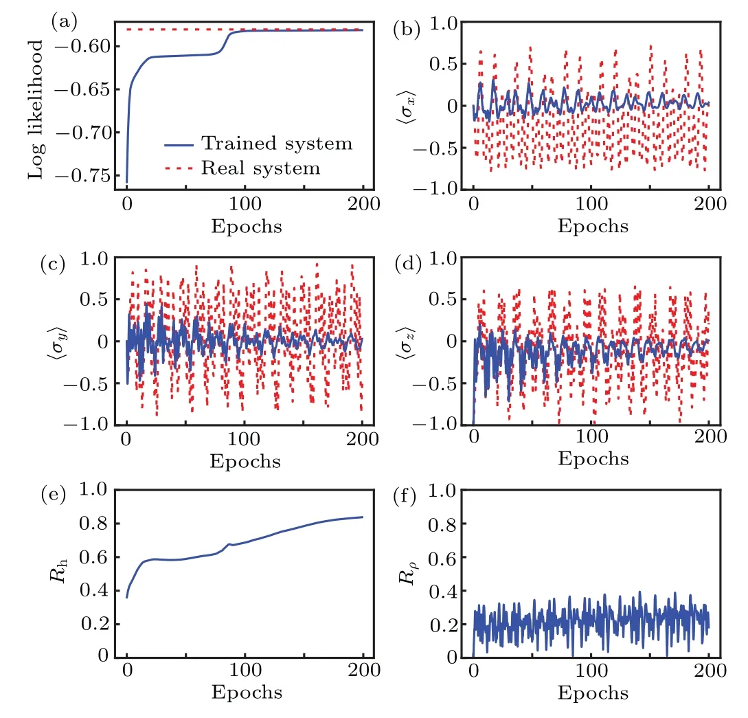
Fig.1. The supervised learning results of an open quantum system. (a)The log likelihoods of trained system and that of the real system. These two curves converge if the training number is large enough. (b)-(d)The dynamical evolution of physical quantities〈σ〉.The blue lines are the learned results and the red lines are the actual values. We see that they do not coincide with other. With the increasing of evolution time, the difference becomes larger and larger. (e)The difference between the learned Hamiltonian and the real one. We see that with the increasing of training time,the difference does not decrease.(f)The difference of density operators between the learned one and the real one.

In order to explain above conflict and check the validity of machine learning,we define

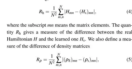
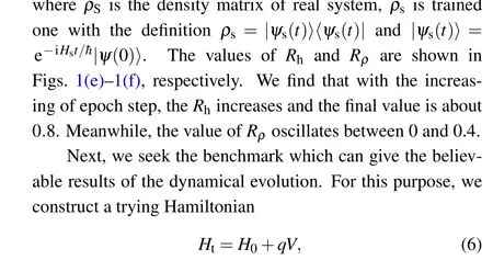
whereqis a small quantity andVis a 8×8 random Hermitian matrix. We note that the generation rules ofVandWare the same except for the dimensions.H0is generated by the same rule Eq. (3) as the real Hamiltonian. Substituting the trying HamiltonianHtinto Eq. (2), we obtain the trying results of dynamical evolution of the physical quantities〈σ〉,which are shown in Fig. 2 as the blue lines with differentq. Here the red lines represent the actual values. We find that only whenqis small enough,the trying results agree with the actual ones.Then we can extract the correct information about the system from the correlation patterns in the series of measurements of the trying HamiltonianHt. Meanwhile,replacing theHsin the measure (4) by theHt, we obtain that if the machine learning works, theRhshould be very small. Figure 2(e) gives the benchmark asRh=1.02×10-5and figure 2(f) gives the benchmark asRh=5.2×10-5. All these values are smaller than that obtained from the learned HamiltonianHs. That is the reason why the learned Hamiltonian can not give the correct dynamical properties of the system.

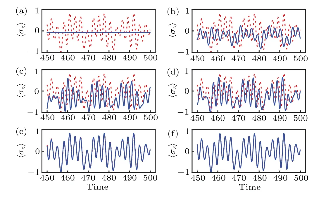
Fig. 2. Dynamical evolution of the physical quantity 〈σz〉. The red lines are the actual values and the blue lines are the results obtained from the trying Hamiltonian Ht with different q. The values of q in panels (a)-(f) are 1×10-1, 1×10-2, 1×10-3, 5×10-4, 1×10-4, and 5×10-5, respectively. We see that only when q is small enough, the trying results obtained from Ht can give the correct dynamical properties of the system. The numerical data of panel (e) give the benchmark as Rh =1.02×10-5 and that of panel (f) give the benchmark as Rh =5.2×10-5. Therefore, if the learned Hamiltonian gives the believable results,the Rh should be small enough.

In order to solve this problem, we use an alternative method which is the dynamic evolution of physical quantities can be learned directly from the dynamical learning,as shown in the following section.

4. Dynamical learning

The expected values of Pauli matrices can also be expressed as

which means that the dynamical properties of physical quantities can also be obtained from the density operator. Thus we carry out the dynamical learning of the density operator directly.

We use a recurrent neural network to realize the dynamical learning, which is a modified version of the echo state network.[39]The neural network constructed in this paper combines the input layer and the output layer to form a loop.[40]Besides the traditional input,our neural network also has a context input, which is used to stabilize the neural network.

The neural network is characterized by

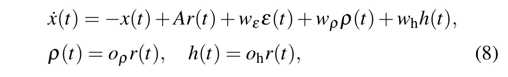
wherex(t) is a function oft,Ais the recurrent weight of the functionr(t)which is related withx(t),wεis input weight of input functionε(t),wρis the feed back weight of the density operatorρ(t),whis the feed back weight of the contexth(t),oρandohare the output weights of density operator and training context,respectively.

We chooser(t)=tanh[x(t)+b] and start from an initial uniform distribution. Thus the initial network parameterswε,wρ,wh, andbare determined by the given initial distribution. The recurrent weightAis a matrix whose elements take the values from 0 to 1. During the learning, only the output weightsoρandohare updated via gradient descent method.The initial values ofoρ,ohare set to zero.

The construction of neural network with dynamical learning includes two steps. The first step is training the neural network. Through training,the neural network will gradually learn how to simulate the dynamic evolution of physical quantities. The second step is testing the network. In this step,the dynamic evolution of physical quantities can be simulated.We note that both of these two steps include the pre-training stage and the dynamical learning stage.

We first train the neural network.We randomly generalize 1000 context matrices{˜h(t)}which have the same structure as Hamiltonian(3). The purpose of this choice is to stabilize the neural network.From these contexts,we obtain the density operators{˜ρ(t)}. The context and the density operators in above sequences are put into the neural network in turn to obtain the training set.

In the pre-training of recurrent neural network, the context and density matrix over a period of time are generated by the continuous measurements of input ˜h(t) and ˜ρ(t). We take the difference between the trained density matrixρ(t)and the input one ˜ρ(t)as the loss function,ε(t)=ρ(t)- ˜ρ(t), to pre-train the neural network. Meanwhile,we use the FORCE rule[41]for online learning to minimize the loss functionε(t)through gradient descent method and to update the output wightsoρandohin the neural network.

After the pre-training,we fix the output weightsoρandohof the recurrent neural network. The contexth(t)in the neural network is also fixed as a constant,which is the average value of all the previously generated contexts in the pre-training process. Next we carry out the dynamical learning. In this stage,we no longer minimize the loss functionε(t)and the weights in the neural network are no longer updated.The network generate the trained density operator and trained context.

From the 1000 training, the output weightsoρandohof the neural network are optimized. The trained density operator tends to the actual value of input one. Because the weights of neural network are fixed, the amount of computation are effectively reduced.

Next, we test the neural network and study the dynamical learning results. Substituting the Hamiltonian (3) in to the neural network and repeating the above pre-training and dynamical learning processes, we obtain the learned result of density operator of the system (3). Based on it, we obtain the dynamical learning results of the physical quantities〈σ〉,which are shown in Figs. 3(a)-3(c). We find that the learned dynamical evolution of physical quantities〈σ〉(blue lines)coincide with the actual values(red lines)very well. Meanwhile,the density operator generated by the neural network is very close to the real one, as shown in Fig. 3(d). Therefore, we conclude that the dynamical properties of the non-Markovian quantum systems can be learned by the neural network with fixed weights.

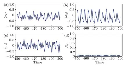
Fig.3. (a)-(c)The dynamical evolution of physical quantities〈σ〉. The red lines are the exact dynamics results and the blue lines are the learned results.We see that these curves coincide with each other very well. Thus the neural network with fixed weights can learn the quantum dynamics. (d)The difference between the learned density operator and the actual value. We see that the difference is very small.

Last, we should note that the Hamiltonian is randomly generated according to the rule(3). The neural network constructed in this paper has the ability to accurately learn other quantum systems including the high dimension cases only if they have the same structure as Eq.(3).

5. Conclusion

We study the dynamical learning of Non-Markovian quantum dynamics by using the neural network with fixed weights. From the generating function of Hamiltonian, we obtain the suitable set of input contexts and the stable neural network. After training, the neural network can generate the learned density operator of a given system very accurately.Based on it,we calculate the dynamical evolution of physical quantities. Comparing with the supervised learning of model Hamiltonian,the dynamical learning results are more accurate.

Dynamic learning has many distinct advantages. For example, it does not need to update the weights of the network during the dynamical learning stage. Thus the amount of computation can be effectively reduced. It avoids the searching of time evolution rule. In some cases, we do not know the Hamiltonian of a dynamical problem. The dynamical learning simulates the dynamical evolution of observable physical quantities directly and the accuracy is very high. We expect that the dynamical learning can be applied to other problems.

Acknowledgements

Project supported by the National Program for Basic Research of the Ministry of Science and Technology of China(Grant Nos.2016YFA0300600 and 2016YFA0302104),the National Natural Science Foundation of China (Grant Nos. 12074410, 12047502, 11934015, 11975183, 11947301,11774397, 11775178, and 11775177), the Major Basic Research Program of the Natural Science of Shaanxi Province,China (Grant No. 2017ZDJC-32), the Australian Research Council(Grant No.DP 190101529),the Strategic Priority Research Program of the Chinese Academy of Sciences (Grant No. XDB33000000), and the Double First-Class University Construction Project of Northwest University.