Qing Yu(虞晴) and Xianbin Liu(刘先斌)

State Key Laboratory of Mechanics and Control for Mechanical Structures,College of Aerospace Engineering,Nanjing University of Aeronautics and Astronautics,Nanjing 210016,China

Keywords: quasi-potential, ordered upwind algorithm, minimum action path, isotropic diffusion and anisotropic diffusion

1. Introduction

Quasi-potentials are a kind of important physical parameters characterizing fluctuational behavior of stochastic systems perturbed by weak noise, which were proposed in the large deviation theory[1]and can describe the difficulty of escape trajectory from one attraction domain, estimate invariant probability distribution and predict mean first escape time. Moreover, a quasi-potential can also be considered as a potential function to quantify stability in stochastic systems.[2,3]It has been applied to investigate fluctuational paths in many stochastic models, e.g., the Maier-Stein model,[4]the Morris-Lecar model,[5]and the FitzHugh-Nagumo model.[6,7]Because of wide application of quasipotentials, plenty of methods to calculate the quasi-potential emerge, such as the optimization approach to construct the quasi-potential for any system described by polynomials,[8]the ordered upwind method (OUM)[4,9]and the ordered line integral method(OLIM).[10,11]

The OUM and OLIM stem from the ordered upwind algorithm,[12,13]which approximates the solution to the static Hamilton-Jacobi equation. To calculate the quasi-potential,this algorithm is then adapted to the stochastic systems by Cameron.[4]Via employing the geometric action functional and the dynamical programming principle,this adaptation can effectively compute the quasi-potential on a regular mesh.Different from the first-order finite difference upwind scheme in the OUM,the OLIM[10]adopts new update rules including the one-point update and triangle update to speed up the calculation,and it is faster than the OUM by the factor of 1.5.

Once the quasi-potential has been computed, the minimum action path (MAP) can also be obtained according to the large deviation theory. Among different noise-induced phenomena,[14-17]the MAP is of concern when one studies how the particle can escape from the basin of attraction or undergo a large excursion.[6,18-21]To check the accuracy of the computed MAP,some existing numerical methods to calculate the MAP are applied. To our knowledge, there are two other major methods to compute the MAP. One method is called the geometric minimum action method (gMAM) by using the geometric action functional.[22]It has been used in many stochastic models[23,24]and there are some variants of the gMAM.[25,26]The other method is to study the Hamiltonian equations derived from the Hamilton-Jacobian equation by using the method of characterization.[27]After obtaining the Hamilton equations,one can compute the escape trajectory from the domain of attraction using the action plot method,[28]the iterative action minimizing method,[29]the adaptive minimum action method[30]and so on. In this work, only the gMAM is applied to examine the accuracy of the computed MAP.

In this paper, a new method to calculate the quasipotential is proposed to save time because the finite difference upwind scheme in the OUM and the triangle update in the OLIM require expensive computational time. This method inherits the “ordered” idea of the ordered upwind algorithm,which means that the quasi-potentials of the mesh points are calculated in an ascending order. Meanwhile,this new method simplifies the ordered upwind algorithm by using the geometric action functional. The update radius and mesh step,which affect the accuracy of the new method,are considered by analyzing a simple linear stochastic system. A general rule for choosing appropriate update radius and mesh step is given.Two cases including isotropic diffusion and anisotropic diffusion are considered. It is found that the new method can effectively calculate the quasi-potential and the MAP for stochastic systems with isotropic diffusion. The anisotropy will pose an important effect on the accuracy of this new method.

In Section 2,the large deviation theory is introduced.The new simplified method is presented in Section 3. Then the method is applied to two stochastic systems in Section 4.Conclusions are drawn in Section 5.

2. Large deviation theory

Consider a stochastic differential equation

whereb(x) is the continuously differentiable vector field,εis a small parameter, the reversibleΣis the noise amplitude tensor, andW(t) is thed-dimensional independent standard Brownian motion.

When the parameterεis small,this stochastic system will spend most of its time in the neighborhood of an attractor,only accidentally far from it. However, when the escape occurs, it will follow one unique optimal trajectory with an overwhelming probability.[1,6]Large deviation theory is a powerful tool to characterize this optimal path.Freidlin and Wentzell[1]connect this path with the extreme value problem of an action functional

Here, the matrixA=ΣΣTis the diffusion tensor or noise intensity tensor,and〈·,·〉denotes the Euclidean inner product.

However, when the initial or end states are equilibria or limit cycles,the timeTin Eq.(2)should be extended to infinite. Then the quasi-potential is introduced as the minimization over both the time and the path:

whereψ(α)is a path connecting two points and the parameterα ∈[0,1]. The corresponding new defined quasi-potential is

Since it is difficult to deal with the infinite time in Eq. (2),we study the quasi-potential in Eq. (6), which considers the minimization over the space of arc-length parameterized curves,[25]and the following computation is based on the geometric action in Eq.(5).

3. Method

Since the quasi-potential in the large deviation theory can determine the optimal path or the MAP, plenty of methods[4,8,10,11]have been proposed,one of which is the ordered upwind method (OUM). The OUM is originally used to approximate the solution to the static Hamilton-Jacobi equation[12,13]and then is adapted to the stochastic systems by Cameron.[4]This method can effectively compute the quasipotential on a regular mesh. Via employing different update rules from the OUM, the ordered line integral method(OLIM)[10]is then put forward, which simplifies the quasipotential calculation and speeds up the computational time.

In fact, both the adapted OUM and OLIM make use of the ordered upwind algorithm. This algorithm divides the mesh points into four categories: unknown points, considered points,accepted-front points and accepted points. Firstly,the considered point with the minimum value of the quasipotential is picked out and label it accepted front. Then update the quasi-potentials of other unknown or considered points with update rules.Then continue to select the considered point with the minimum quasi-potential until the point reaches the boundary. Since a Hamilton-Jacobi equation for the quasipotential can be obtained by employing the dynamical programming principle,[4]the ordered upwind algorithm can effectively calculate the quasi-potential. In addition,the update rules for the quasi-potential are based on the Hamilton-Jacobi equation. However,if the update rules are chosen just according to the geometric action functional in Eq.(5),the algorithm itself can be further simplified.

Firstly, the mesh points are divided into three categories and the accepted-front points are not necessary:

Unknown point the point where the quasi-potential has not been computed yet.

Considered point the point where the tentative quasipotential has been calculated but the value of it has not been determined.

Accepted point the point where the quasi-potential has been determined.

Note that there are some differences of the definitions of the points between the new method and the OUM.[4,10]Then the outline of the simplified ordered upwind method is as follows:

Step 1 Make all mesh points unknown. Compute the tentative quasi-potentials at mesh points in the nearest neighborhood of the attractor and make them considered.

Step 2 Find the considered pointx*with the smallest tentative values and relabel it as accepted. If this point is on the boundary,then the procedure terminates.

Step 3 Update the quasi-potentials of all unknown and considered points within the rectangular centered atx*with a reasonable length 2KΔxand width 2KΔy. And label all unknown points that have just been calculated considered. Then go to step 2.

Here the mesh stepsΔxandΔyare the smallest distance between two adjacent mesh points inxandydirections, respectively. Different from the mesh size in Ref.[4],the mesh step is considered here for convenience of analysis. Meanwhile,the update radiusKis not chosen to makeKΔthe maximum distance from one point,but adopted to letKΔthe half side length of the rectangle centered at one point, as shown in Fig. 1. The appropriate update radiusKand mesh stepΔfor this new method are determined in the following. In addition,note that this new algorithm inherits the“ordered”idea of the OUM, which means that the quasi-potentials of the mesh points are calculated in an ascending order.

Fig.1. The different update radii K.

Before analyzing the update radius and mesh step, one important point should be noted. According to the large deviation theory,once all quasi-potentials in one area are obtained,the MAP of every point in this region can also be acquired accordingly. Since the MAP is of concern in most stochastic situations,the purpose of this new method is to make the computed MAP as accurate as possible with less computational time. Therefore, the effectiveness of the new method will be checked by analyzing the computed MAP. If the system under study is of no analytical quasi-potential, among different methods to calculate the MAP, the path calculated by the geometric minimum action method (gMAM)[22]is chosen as a reference.

To get the appropriate update radiusKand mesh stepΔ,consider a simple linear stochastic system which has been proposed in Ref.[10]:

where the quasi-potentialU(z1)has already been determined and ˜U(z) denotes the tentative value of the pointz. This first-order integral rule is similar to the one-point update in the OLIM,but the tedious triangle update in the OLIM is not necessary for the new method.

Since this linear system has a symmetrical structure, the computational domain is confined in the square[-1≤x ≤1]×[-1≤y ≤1] and the mesh stepΔxandΔyare chosen to be the same. As shown in Fig. 2(a), for allΔx,the maximum absolute error between the analytical quasipotential and the one calculated by the new method will decrease as the update radiusKincreases. For all values of mesh stepsΔx, whenKis small, the errors will remain large. The fact that only the increase ofKcan reduce these errors indicates that the accuracy of the new method is more relative to the update radiusKthan the mesh stepΔx. Moreover,the errors start to vary slowly when the radiusK ≥14. This means that effect of larger values ofKon the accuracy will decrease.However, the changes of the error to the mesh stepsΔxin Fig.2(b)are different from the former figure.When the update radiusKis small, the error will increase as the mesh stepΔxdecreases. Then asKincreases,the error starts to drop. In addition,note that whenK=15 and 20,the differences between errors of these two situations are very small and almost indistinguishable. Therefore,the sufficiently large update radiusKand small mesh stepΔxcan guarantee enough accuracy.

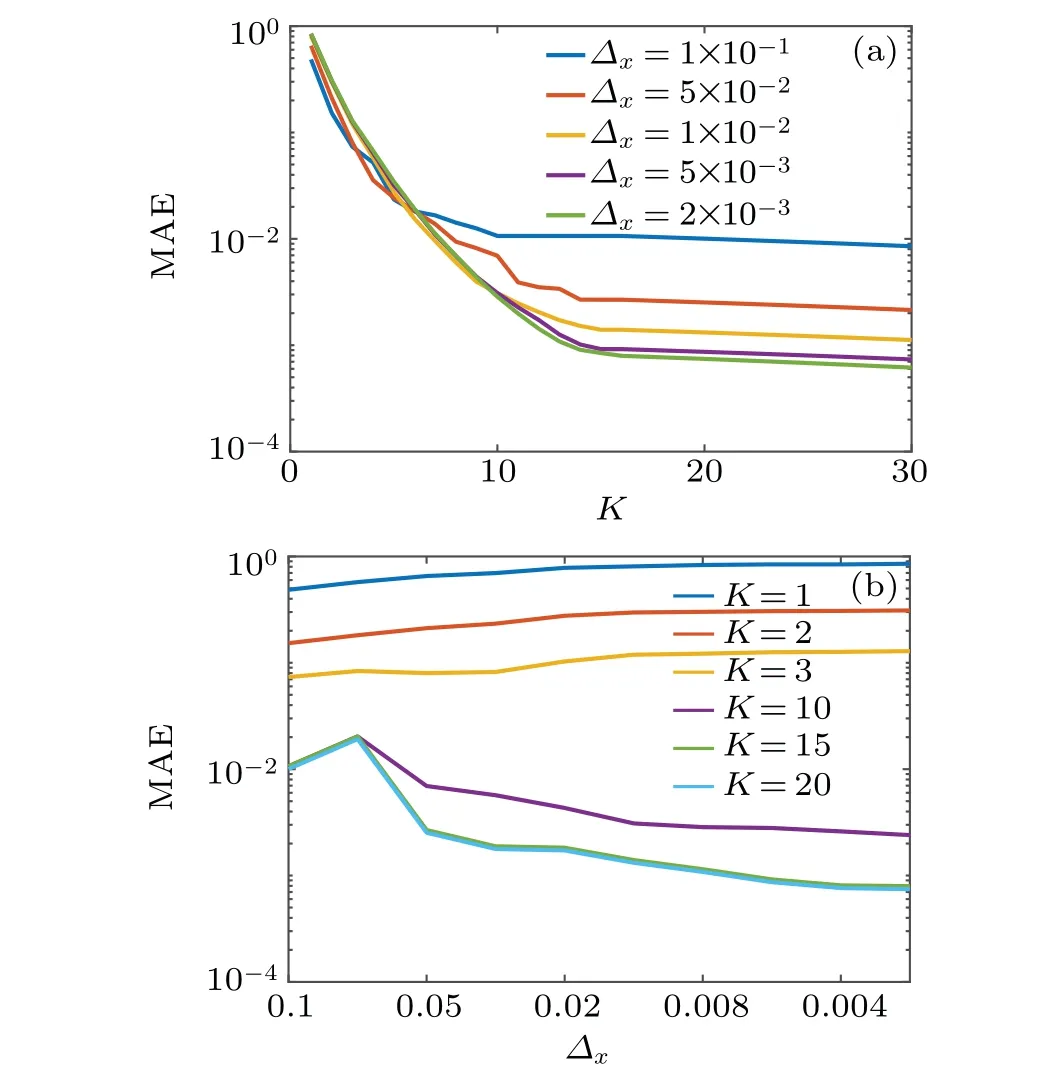
Fig. 2. The maximum absolute error (MAE) of the update radius and the mesh step Δx. (a) The change of the error to the update radius K.(b)The change of the error to the mesh step Δx.

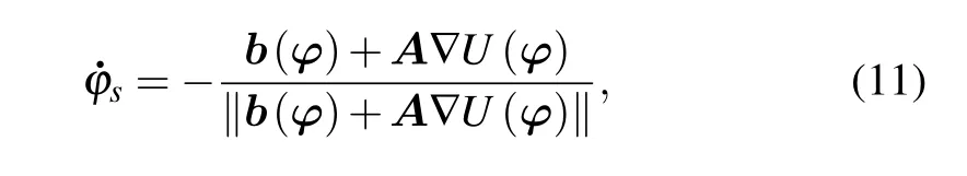
However, note that the MAP is of concern in this paper.Once the quasi-potential is computed,the MAP can be calculated according to the following equation:[4,11]

where the trajectory is shot from the arrival point, which means that the reverse integration is applied to obtain the fluctuational path. In Fig. 3(a), the exact and the computational MAPs agree well with each other when the mesh stepΔx ≤0.02. In fact,whenΔx>0.02,the MAP cannot be computed by Eq.(11)because the mesh is too coarse to calculate accurately the gradient of the quasi-potential,i.e.,∇U(φ). In addition, Fig. 3(b) depicts several MAPs for different update radiusK, where the mesh stepΔx=0.01. WhenKis small,there are obvious differences between the exact and the computed MAPs. However,these paths can be barely distinguishable when the radiusK ≥5.

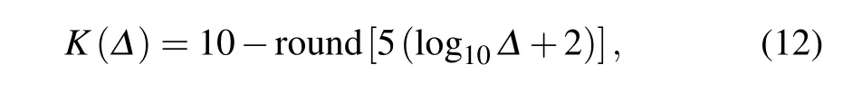
Then based on these numerical analyses and suggested update radiusKin OUM and OLIM,[4,10]to calculate the accurate MAPs, one can choose the update radiusKaccording to the following empirical equation:

whereΔis the mesh step,which is smaller in thexandydirections. In addition,for the mesh stepΔ,when the boundary is of orderO(1), which is the interval[-1≤Δ ≤1]in this linear system,the stepΔshould not be more than 0.02.To obtain more accurate results,one can choose the smaller mesh step at the cost of the computational time, which is discussed in the following. Furthermore, we should note that if the boundary is of orderO(0.1),the mesh step should be rescaled.

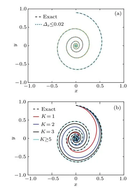
Fig.3.The exact and the computed MAPs for the linear system arriving at the point(0,0,9). (a)For K=10 and all Δx ≤0.02,the exact and the computed MAPs agree well with each other. (b) The different MAPs for different values of K when Δx=0.01.

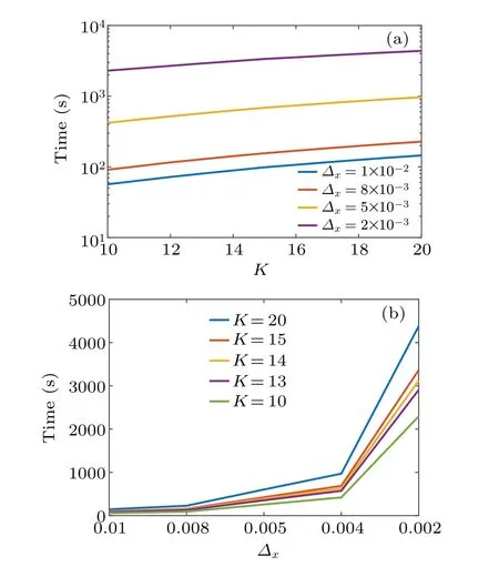
Fig.4. Computational time consumed by the new method. (a)The variation of the time to the update radius K. (b)The change of the time to the mesh step Δx.

After the reasonable update radiusKand mesh stepΔare presented,we can continue to evaluate the computational time of the new method and compare this new method to the other existing methods including the OUM and OLIM. In Fig. 4,the variations of the computational time to the update radiusKand mesh stepΔxare depicted. AsKincreases andΔxdecreases,the consumed time grows monotonically. In addition,as shown in Fig.4(b)where the scale of theycoordinate is linear,for all values ofK,the consumed time is small whenΔxis large and will start to increase dramatically whenΔx<0.004.Therefore,the time is more related to the mesh stepΔxthan the update radiusK,which is different from the relation between the accuracy and the two factors.

Fig.5. (a)The maximum absolute errors of the mesh step for the three methods.(b)The computational time for the three methods.The update radius is chosen according to Eq.(12).

Since the mesh step will greatly influence the computational time,the relations between the mesh step and computational time for the three methods are depicted in Fig.5(b). It can be observed that the new method is faster than the OUM and OLIM.The least-square fit to the formulaT=CΔ-qfor the computational time is given in Table 1. These numerical results show that the new method is faster than the OLIM by the factor of nearly 12. Moreover, the maximum absolute errors between these methods are displayed in Fig. 5(a). The new method is more accurate than the OUM and otherwise is slightly less accurate than the OLIM. As shown in Table 1,which also gives the least squares fit toE=CΔqfor the error,the new method is near 80 times more accurate than the OUM and the OLIM is more accurate than the new method by the factor of near 1.5. However, the new method can still effectively calculate the quasi-potential and the MAP whenKandΔare chosen appropriately. Therefore these numerical results illustrate that under enough accuracy,the new method has the advantage of time-saving strategy.

This section discusses a new simplified OUM to compute the quasi-potential and the MAP.Different from the OUM and OLIM, this new method adopts a simplified algorithm which inherits the“ordered”idea of the ordered upwind algorithm.In addition,the first-order line integral rule is used as the update rule in the new method. This rule is similar to the one-point update rule in OLIM, but the triangle update of the OLIM is not used, which will cost much time because the triangle update involves the problem to root finding of equations. The new method can both speed up the calculation time and maintain sufficient accuracy. Note that this new method is designed for systems with isotropic diffusion. Then the effectiveness of this new method for systems with isotropic diffusion will be checked in Section 4 and the extension of this method to systems with anisotropic diffusion will also be investigated there.

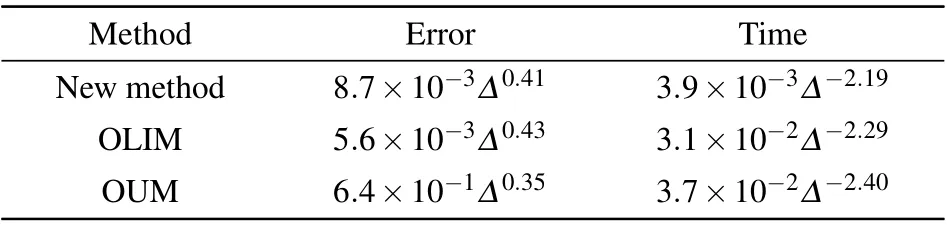
Table 1. The least squares fits to the formulas E=CΔq and T =CΔ-q for the maximum absolute errors and the computational time.

4. Stochastic systems

4.1. Isotropic diffusion

The new method presented in Section 3 is applied to the system with isotropic diffusion in this subsection and the other case is discussed in Section 4.2. Once quasi-potentials in a region are computed, the MAP of every point is also obtained.With the computed MAP, one can study the escape behavior from the domain of attraction of an attractor.

To investigate the escape path, we consider the Maier-Stein model[31]with the parametersµ=1 andα=10:

This system has three fixed points: two stable points (±1,0)and one saddle(0,0).Since the deterministic Maier-Stein system is symmetrical about theyaxis, only the right half planex>0 is considered here. This means that the escape behavior from the domain of attraction of the stable fixed point (1,0)is studied. According to the large deviation theory, the escape trajectory will move out of the attraction domain through the saddle point(0,0). Therefore,the escape trajectory is the MAP connecting the stable point (1,0) to the saddle point(0,0). As there is no analytical quasi-potential for the Maier-Stein model, the MAP computed by the new method is compared with the one calculated by the gMAM, which is an effective method to obtain the fluctuational path.

For the computational domain,we first choose a large domain and observe the distribution of the quasi-potential. Under the condition that the quasi-potentials in the vicinity of the saddle point have been calculated, we reduce the domain to refine the mesh and to improve the accuracy. The final domain is confined in the square[-1.5≤x ≤1.5]×[-0.7≤y ≤0.7]for this Maier-Stein model. Because the boundary values areO(1),the mesh step can be chosen asΔx=0.01 andΔy=0.01.Then the corresponding update radiusK=10.To compute the escape path by Eq.(11),(0.001,0.001)is chosen as the initial point.

Figure 6(a)displays the distribution of the quasi-potential in the phase space. The two escape paths calculated by the new method and the gMAM coincide well with each other,which can be seen clearly in Fig.6(b).This agreement demonstrates that the new method is an effective method to calculate the quasi-potential and the MAP. In Fig. 6(c), an overall appearance of the quasi-potential in 3D is also depicted. The quasi-potential is minimum at the stable point (1,0). Moreover,along thexaxis fromx=1 tox=-1,the quasi-potential increases until reaching the saddle point (0,0). Then it remains unchanged to reach the stable point (-1,0). This is evident because the escape trajectory only needs to overcome the potential barrier between(1,0)and(0,0). Once this path reaches the origin, it will follow the deterministic flow to the other stable point(-1,0)with no extra quasi-potential needed.

Fig.6.The quasi-potential and the escape trajectories from the domain of attraction of the stable point(1,0).(a)The quasi-potential distribution is denoted by the color code. Two extra red solid line and blue dashed line represent the trajectories calculated by the gMAM and the simplified OUM,respectively. (b)The enlargement of the two paths in(a). (c)The 3D distribution of the quasi-potential.

4.2. Anisotropic diffusion

For systems with anisotropic diffusion, it is found that anisotropy will affect the accuracy of the OLIM.[11]Therefore, we extend the new method to systems with anisotropic diffusion and observe the effect of the anisotropy on the computed MAPs.

Consider a simple fast-slow system with anisotropic diffusion[24]

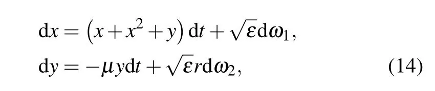
where the parameterµ=0.01, and the parameterrcontrols the noise intensity tensor. The deterministic system contains two fixed point: one stable point (-1,0) and a saddle point(0,0).

For this fast-slow model, the computational domain is confined in the rectangle[-1.5≤x ≤0.2]×[-0.3≤y ≤0.3].Since the boundary isO(0.1),the mesh step can be chosen asΔx=0.001 andΔy=0.001. Here for the sake of time saving,Δx=0.002 andΔy=0.001 are adopted as the final mesh steps.Then we consider four values of the parameterr:

Whenr=1, which corresponds to the isotropic diffusion, to compute the escape path from the stable point (-1,0) to the origin,(-0.030,0.029)is chosen as the initial point.However,for the other values ofr,(-0.01,0.0099)is chosen as the initial point in this study. In addition, the initial quasi-potential calculation around the stable point(-1,0)is presented in Appendix A.

Fig.7. The quasi-potential and the escape trajectories when the parameter r=1. (a) The quasi-potential distribution is denoted by the color code. (b)The enlargement of the two paths in(a).

Figure 7 depicts the quasi-potential and the escape paths for the isotropic diffusion. The two escape paths calculated by the gMAM and the new method are consistent with each other. However, this phenomenon is not always true for the anisotropic diffusion. Forr=0.07 in Fig.8, these two paths still coincide a bit well. Then for the case ofr=0.05, the differences on the middle horizontal lines appear. Moreover,whenr= 0.03, there is an obvious gap between these two paths. In fact, on the middle horizontal lines of the escape paths, there is about 0.0041 deviation in theydirection between these two paths. This numerical discrepancy means that when the new method is applied to systems with anisotropic diffusion, the noise intensity tensorA=ΣΣTwill have an important effect on the accuracy of the computed MAP.

Fig.8. The quasi-potentials and escape trajectories for different values of the parameter r.

Note that the ratio of the maximum eigenvalue to the minimum one of the noise intensityAis

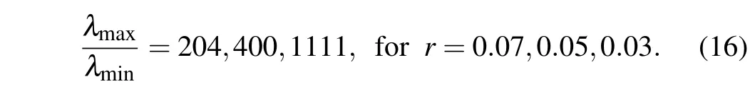
Therefore, as the ratioλmax/λmingrows, the MAP computed by the new method will gradually deviate from the actual MAP. This phenomenon is similar to that observed in the OLIM.[11]Thus,for numerical methods based on the ordered upwind scheme,the anisotropy will affect the accuracy of the computed quasi-potential and MAPs. However, if the ratio is not large, the new method can still effectively compute the MAPs. In addition, even if the ratio is large, the computational path can be used as a reference for the actual MAP or as an initial curve for the gMAM,which has local convergence.

5. Conclusion

This paper presents a new method based on the ordered upwind algorithm to obtain the quasi-potential of stochastic systems.This new method simplifies the ordered upwind algorithm and adopts the first-order line integral as the update rule.In addition,the new method speeds up the computational time and is faster than the OUM and OLIM.Two factors including the update radiusKand mesh stepΔare investigated by analyzing a simple linear stochastic model. Through numerical analyses, it is found that the accuracy of this new method is more related to the update radiusKthan the mesh stepΔ,but the computational time is reverse. This new method can effectively compute the quasi-potential if these two factors are chosen appropriately. Therefore for stochastic systems with isotropic diffusion, a simple general rule is then given, based on which the quasi-potential and the MAP can be computed effectively with only a small amount of time.

The new simplified OUM is then applied to stochastic systems with isotropic diffusion and anisotropic diffusion. It is found that this method can effectively calculate the MAP for the Maier-Stein model with isotropic diffusion. For the fast-slow system with anisotropic diffusion,the numerical results show that if the ratio of the maximum eigenvalue to the minimum one of the noise intensity tensor, i.e.,λmax/λmin,is not large,the new method is still useful to calculate the MAP.However,if this ratio is large,there is an obvious gap between the paths calculated by the new method and the actual MAP even if this error is small.

In a nutshell,in this paper,a new method,which can accurately calculate the quasi-potential and the MAP for stochastic systems with isotropic diffusion and greatly reduce computational time,is presented.It is found that the anisotropy will affect the accuracy of the computed MAP.Since we mainly deal with the two-dimensional vector field with Gaussian noise,the extension of this method to higher-dimensional systems or multiplicative noise and non-Gaussian noise will be studied in the future. In addition,as the geometric action requires the reversibility of the noise intensity tensor, OUM and the new method fail to deal with irreversible or unilateral noise. Therefore the adapted or new theory is expected to be proposed to deal with these particular situations.

Acknowledgements

This work was supported by the National Natural Science Foundation of China (Grant Nos. 11772149 and 12172167),the Project Funded by the Priority Academic Program Development of Jiangsu Higher Education Institutions (PAPD),and the Research Fund of State Key Laboratory of Mechanics and Control of Mechanical Structures (Grant No. MCMS-I-19G01).

Appendix A:Initialization of the new method