Hao-Wen Wang(王浩文) Yun-Jia Xue(薛韵佳) Yu-Lin Ma(马玉林)Nan Hua(华南) and Hong-Yang Ma(马鸿洋)

1School of Sciences,Qingdao University of Technology,Qingdao 266033,China

2School of Information and Control Engineering,Qingdao University of Technology,Qingdao 266033,China

Keywords: quantum error correction,toric code,convolutional neural network(CNN)decoder

1. Introduction

Since qubits are not independent in quantum computers,[1]they will interact with the external environment during operation,thereby destroying the entangled state between qubits and causing quantum collapse.[2]In order to overcome the influence of noise caused by quantum incoherence, the emergence of quantum error correction codes is an important technology to solve the problem of noise. According to the theory of quantum error correction(QEC),[3-6]if the interference intensity generated by noise is less than a certain threshold,the logical qubits encoded with physical qubits can be well protected.

In order to make the interference of noise intensity closer to the threshold level in the experiment, finding a quantum error correction code with excellent performance is crucial.The stabilizer formalism[7]is a powerful technique for defining and studying quantum error correction codes based on the Pauli operator. It can directly analyze the symmetry of the code,perform error detection and correction,and describe the most widely used form of topological codes.[8,9]The stabilizer code is a quantum error correction code defined in the stabilizer form. It consists of two sets of operators. One set is a stabilizer generator and the other set codes logical operators.The stabilizer code can detect errors by measuring the information of the stabilizer operator, without changing the coded information,[10]so that the qubit information is not detected and collapsed.

Next, we analyze the error information detected by the stabilizer operator[11]and perform a recovery operation to correct the error. The appearance of the decoder allows researchers to find a suitable error correction from the available classical data,that is,the output of the stabilizer operator measurement[12,13]result in the form of±1 is called a decoder.We need to find the result that the optimal decoder reaches the output threshold close to the optimal threshold. For the determination of the best decoder, the decoding calculation under the simplest noise model such as the depolarization noise model is also a very difficult problem.Therefore,we try to find a code with a good constrained structure.[14]The appearance of topological code[15-19]provides us with great convenience in decoding calculations. It has a stable generator with local support, and its stabilizer is geometrically locally, to characterize any return-1 measurement result that does not meet the constraints of the stabilizer. The result indicates that there is an error in the qubits near it. Using this scheme, we can effectively decode. In the choice of decoder,we use the CNN network structure to provide great convenience for the following toric code error correction.

2. Toric codes in dual space

2.1. Quantum toric error correction code under the plane

Toric code[20-22]is a quantum error correction code with good periodicity proposed earlier. Its typical representative is that the quadrilateral lattice conforms to the self-dual and boundary roughness, which perfectly conforms to the error correction. The code requires regularity and periodicity for error correction in handling error types. In addition, it is the simplest topological code with good local stability,which also provides a guarantee for it as a good error correction code.The square is embedded in the toric torus,so that the leftmost edge is marked on the rightmost side,and the uppermost edge is marked on the bottom edge. As shown in Fig. 1, the lattice consists of vertices(points where edges intersect),lattices(closed quadrilaterals surrounded by edges), and boundaries(consisting of edges on the edges of the lattice). Among them,boundaries,vertices and grids play a key role in the error correction process.

Among them,Rrepresents a type of logical operator, which is composed of multiple physical qubits,Prepresents a stable generator, which is composed of the tensor product of multiple Puli operators,LIis one of theRlogical operators group,and it characterizes the stability of logical qubits. We embed qubits on each side of the lattice (represented by green circles in Fig. 1). On theL×Llattice with periodic boundary conditions, we have 2L2edges. When calculating the boundaries, care should be taken not to count repeatedly(in Fig.1,the edges of the edges are represented by gray circles). From this,we can calculate that the toric code hasn=2L2physical qubits. Corresponding to the foregoing, in the toric code, the vertices and lattices on the lattice constitute two stable generators,which are define as follows:ALandBPare vertex operator and plaquette operator:

among them,jrepresents the edge,and bothXandZare Pauli operators. The plaquette operator is composed of the tensor product[23,24]of the PauliZoperator acting on the 4 qubits of the lattice boundary, as shown in Fig. 1. The vertex operator consists of the tensor product of the PauliXoperator acting on the 4 qubits adjacent to the vertex. According to the characteristics of stable generators (see Eq. (1)), all operators must be in reciprocity(to ensure that they are not affected by the order in which errors occur),so all plaquette operators in the lattice are reciprocal, and so are all vertex operators. More importantly, adjacent plaquettes and vertex operators are also commutative(the two adjacent ones have two overlapping edges),but non-adjacent lattices and vertex operators are not commutative,because they are in different qubits forming a non-trivial ring.[25,26]

Fig. 1. The toric code is a lattice with a boundary after the circular surface located inside the torus is mapped to the plane. The square is embedded in the toric ring,the leftmost side of the square is connected to the rightmost side of the square,and the uppermost side is connected to the rightmost side, so we only identify one side. Among them, 4-qubit Pauli Z can form a vertex operator and 4-qubit Pauli X can form a plaquette operator.

2.2. Toric code mapping under dual lattice

The plane lattice (also called primitive lattice) is given above. We move the plane lattice up and down by half a unit to generate the dual lattice.[27,28]The dotted line indicates the formation of the dual lattice as shown in Fig.2. The plane lattice has the same size and boundary,but according to the mapping relationship of the dual lattice, we define as follows: A dual latticeΛof latticeΛ∨is a set of vectorsX ∈span(Λ)and satisfies∀v ∈Λ:x,v ∈Z.If we add a linear transformation[29]to the original lattice(here is rotation),then the dual lattice of the new latticeRΛcan be obtained by rotating the original dual lattice(RΛ)∨=R(Λ)∨. We find that no matter what kind of lattice is,its dual lattice has the following relationship with it:

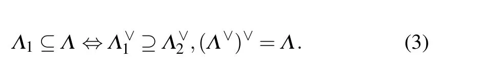
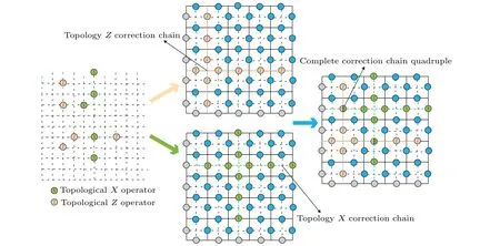
Fig.2. Choose a 5×5 toric code,where the dotted line represents the dual double lattice after the plane lattice. Move up and down by half a unit,the circle represents the physical qubit,the gray circle represents the period. The boundary,the dual double lattice is on the dual lattice.Topological operators X and Z each form a topological correction chain on the dual double lattice. Finally,the topological correction chains of X and Z are combined to form a complete correction quaternion. The local stability of the topology is used to facilitate the stable progress of quantum error correction.

Therefore,we have a characteristic that the dual lattice is the“reciprocal”of the original lattice. Returning to our toric code under the dual dual lattice, its vertices are the lattices of the plane lattice,[30,31]and vice versa,corresponding in the Pauli operator,the PauliXoperator under the dual double lattice corresponds to theZoperator of the plane lattice,and the PauliZoperator under the dual double lattice corresponds to theXoperator of the plane lattice. The dual double lattice plays an important role in the toric code. We can choose the most suitable lattice for our calculation to describe the vertices of the original lattice,which greatly simplifies the calculation process.[32]For example, in Fig. 2, we can choose a suitable small grid to understand the tensor product of the operator.We choose the square as the carrier for studying the toric code.An important reason is that the dual of the square is also a square.We call this the dual grid to be self-dual, and this feature is very suitable for equal protection of topology codes withXandZerrors.

3. Quantum error correction and CNN decoder framework

3.1. Error detection

Error detection[33]is carried out by measuring the output result of the stable generator.When there is no error,the stable generator will output an eigenvalue of+1. When an error occurs,the constraint condition[34]of the stable generator is not met, and the output is-1 eigenvalues. For the measurement of stable generators, we do not need to measure all generator groups, i.e., 2m, because the properties of each group of stable generators will ensure the independence of each group of stable generators. Therefore, we only need to measureN-Kstable generators,and the number of measurements is linearly proportional to the number of physical qubits. When we find the location of the error, the next step is the error correction process.

We defineQas the Pauli error operator.[35]If it is in a pairwise relationship with the stable generatorS,then we can set|ψ〉as the initial state before the error occurs,so

It can be seen that the stateQ|ψ〉after the error is the-1 eigenvalue ofS. Since we only consider the errors caused by Pauli operator (because the measurement of the stabilizer operators projects converts more general errors into Pauli errors),any two Pauli operators withn-bit qubits are either commute or anti-commute[36]easy, so all error cases are suitable for our analysis above. For simpler noise models, the processing of depolarized noise models[37]is independent and the generation of each error type with the same distribution isPX=PY=PZ=Peff/3. Among them,peffis the error rate characterizing the error correction capability. Since different errors will produce the same syndrome,the equivalence class members of logical operators are the main reason for the impact.

Fig.3. The two strings(red and yellow in the figure)formed by the Z error on the original lattice can form the same syndrome. In the stabilizer,errors can be corrected and combined into a set of closed loops toform a stabilizer operator.

3.2. Error correction

We can regard the syndrome as a charged quasiparticle.[38-41]When the measurement output is +1, the charge is 0(we call it no particle). When the measurement result is-1,the charge amount of 1 is the quasiparticle related to the vertex and the grid. According to the error correction rules,theZerror in the error-free state will create a pair of+1 charged quasiparticles at adjacent vertices. When an error occurs,theZerror adjacent to the+1 quasiparticle will move the quasiparticle to the case that,if the error is adjacent to another vertex, then another quasiparticle is moved here, they will be annihilated,and the qubit at the vertex will be in a zero charge state,thus achieving an error correction process. As shown in Fig. 3, the error correction capability also depends on the intensity and type of errors. We define the error correction and elimination rules of toric codes as follows:

among them,the subscriptkrepresents the excited state at the toric code grid,and the subscriptmrepresents the excited state at the vertex. From this,we can conclude that the excited state of the error particle is generated in pairs to form a closed loop for the excited state annihilation. Can be generated individually,which will cause errors that cannot be corrected.

In the past, we can determine the appropriate syndrome according to the statistical mapping method. However,due to the strong spatial correlation between the grid and the vertices of the toric code,it is difficult for us to use the usual statistical methods to select[42]to make selections. Therefore, we now propose a machine learning-based CNN decoder to determine the best syndrome more quickly,and continue to optimize the conditions to achieve the maximum good threshold. Given errorQand stabilizer elementS,when the errorsQandSQlead to the same measurement result(produce the same syndrome),we need to automatically select the error correction operator from a set of stabilizer measurement results,which is called a decoder,[43-45]as shown in Fig.4.

Fig.4. Z will generate two pairs of green syndromes at the four adjacent vertices,and X will generate a pair of upper and lower red syndromes.When two syndromes of the same type generated by errors appear in the same position,they will cancel out.When different types of syndromes appear in the same position,they will be marked as new yellow syndromes.

3.3. Convolutional neural network architecture

Convolutional neural network consists of three structures:convolution,activation and pooling. The reason why the CNN model can be designed by using the strong spatiality in the image is that the grid and vertices of the toric code have a strong correlation, and the feature space (syndrome) will be used as the input of the fully connected neural network. The fully connected layer is used to complete the mapping from the input feature space to the label set(recovery operator after error correction), that is, to achieve the classification effect. In the early stage of the experiment(or operation),we will train the neural network decoder,starting with smaller data and shorter code distance,[46,47]and when the training threshold is close to the optimal threshold we want,we will expand the amount of data. At the same time,the expansion of the amount of data will lead to an increase in training time and the requirements for the machine will be particularly high. Therefore,we must reduce the cost of training by optimizing various conditions of the CNN network structure. CNN achieves the training effect by iteratively adjusting the network weights through training data,which is called a backward propagation algorithm,[48]as shown in Fig.5.

Fig.5.The input is mapped to the convolutional neural network from the dual dual lattice with vertices and plaquette dual channels respectively.A certain size of convolution kernel is selected in the convolution layer. If it is wrong in the output layer,the eigenvalue of the output is+1. If it is wrong,the output eigenvalue is-1.

We clearly know that the training of the correction process as a classification is a supervised learning,[49]our loss function is the classification cross entropy[see Eq.(7)]. In order to ensure that the value obtained during each classification cross entropy can be best close to the true value,we introduce the currently popular Adam optimizer.[50,51]On the one hand,it performs gradient descent after each iteration of entropy to prevent local optimal conditions. To avoid the phenomenon that the error is too large, on the other hand, the normalization process can minimize the loss function. Due to the large number of iterations and the huge amount of data,we use the RestNet network[52,53]structure in the CNN network. This architecture makes a reference(X)for each layer of the iteration and learns to form the residual function. We pass 7 or 14 iterations,after that,the residual block will be obtained,which will reduce the dimensionality of our convolution operation, thus ensuring the improvement of the iteration speed, and further reducing the dimensionality of the convolution kernel, which can increase the iteration depth by 50%, a good convolution effect can be achieved. This is achieved by introducing the remaining shortcuts,connecting to perform identity mapping,and skipping stacked layers. The shortcut output is added to the output of the stacked layer, and when moving from one stage to the next,the number of filters is doubled.the syndrome that can successfully mark various error rates[54]below the threshold. Since syndromes with a higher error rate are generally more challenging for classification, it is desirable to train the neural network mainly in a configuration corresponding to an error rate close to the threshold. First, we train with a small code distance through the collected data set,choosing RestNet7 and RestNet14 as the network architecture,and the prediction model is generated on this lower error rate data set.

Then we increase the code distance,use a data set with the same error rate for prediction training,and stop training when we are close to the threshold. Finally,when the code distance is increased again,we can find that the prediction result of the data set with the same error rate is far from the threshold value,which means that we have trained the prediction model closest to the threshold value under this data set. As shown in Fig.6,the prediction model under the smaller code distance is still far away from our training model. Through further optimization,as shown in Fig.7,we find that the error rate of the prediction model is almost the same as our training error rate.[55]Consistent in Table 1,we provide the training data set,the number of iteration steps and the accuracy rate,and then use the training model to correct the detection process.

Fig.6. The accuracy of the RestNet7 network layer is much lower than that of the prediction model when the number of samples is small. With the continuous increase of training samples,the prediction accuracy approaches the training accuracy, which can get about 65.547%, better predicting the model we need.

where→yiis the classification bit string for input→xi,→f(xi)is the likelihood vector returned by the neural network.

3.4. Training

In order to better predict the correction model,we need to train the data set through the CNN network model, and train

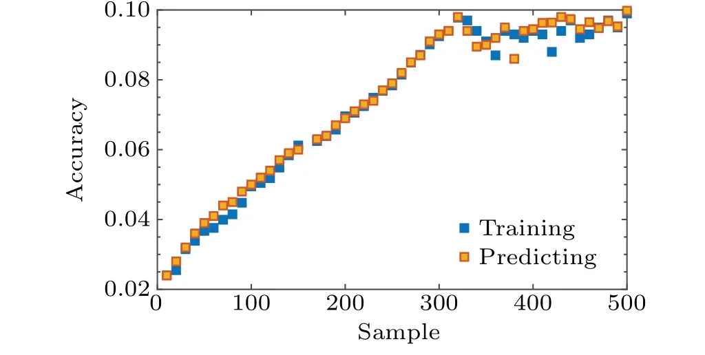
Fig. 7. Compared with RestNet7, the RestNet14 network layer has a better fitting effect in accuracy. A very good prediction can be achieved from the first few samples, but the accuracy is low. When the number of training samples continues to expand,the accuracy can be 65.987%in increase. Because the code distance and the influence of external factors are also involved,when the code distance is increased,the prediction accuracy rate reaches a saturation level.

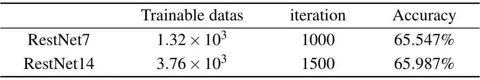
Table 1. The accuracy of prediction model.

3.5. Result

When we correct and predict the trained convolution model,we need to do some processing on the convolution. As shown in Fig. 6, in order to ensure the boundary and periodicity of the grid after each step of convolution,we need to fill it regularly. First assign a random error ratepeffto each edge.Then,we sample the errors based on the error rate of each edge and calculate the syndrome. In the process of correction, we usepfailto characterize logical errors and find their intersection with different code distances. We draw the threshold of the CNN decoder under the depolarization noise model.[56]In Table 2 we give the training parameters, steps and thresholds under different code distances. From the table, we can conclude that as the distance of the code increases,the accuracy of the correction will increase. However,due to the influence of the amount of data and training time,the threshold will reach a saturation level,and increasing the amount of data again will have the opposite effect.

Table 2. Different code distance thresholds.

Under the code distance ofd=3 andd=5 in Fig.8,the logic error rate[57]rises faster at the beginning and reaches the threshold level later. Therefore, when we increase the code distance, we must also consider the amount of training data and the effect of correction time. When we increase the code distance but do not increase the amount of training data, as shown in Fig.10,we can see that the initial effective error rate rises relatively slowly, and the training speed is also limited and increases with the code distance. When we increase the training data set,it can be seen that the initial logic error rate increases faster than Fig. 9 with the increase of the effective error rate function, but the two curves are basically flat when thepeffreaches about 0.18.

Fig. 8. Under the code distance of d =3, 5 and 7, the logic error rate shows a gentle increase. There is not much difference in the growth rates for the three curves,and the threshold level can only reach about 3.5%,which is still far from our ideal optimal threshold.

Fig.9. Under the same code distance,we switch to the RestNet14 network layer. It is obvious that the logic error rate has a rapid increase in the initial trend,and the threshold level has also been well improved,reaching about 5.9%.

Fig.10. When we increase the code distance,d=5,7 and 9,the logic error rate is initially higher than before. However, the error rate will slowly increase when it reaches the middle position, until it reaches a plateau and the threshold is raised to about 8.9%.

In Fig. 11, we increase the data set while increasing the code distance.[58-60]It is obvious that the logic error rate ofd=9 is significantly higher than the other three pictures,and it can reach the threshold level faster. However,as thepeffincreases, the logic error rate tends to be stable, and increasing the data set again will have a reduced effect.

Fig.11. In order to further improve our threshold level,while increasing the code distance, we also replaced the high-accuracy RestNet14 network layer. It can be clearly seen that the logic error rate has a larger threshold in the initial stage. As peff increases, our threshold level approaches 10.8%,and we have the ideal threshold level we need.

4. Conclusion

We still have a long way to go in our search for quantum error correction. We need more powerful code support to solve the impact of complex noise models,and the increase in code distance beyond the threshold limit will lead to low proficiency of error correction. Therefore, we need to find more powerful algorithm support in the optimization of the decoder,and we also need to develop more sophisticated instruments in terms of the accuracy of the training process. Mature neural network decoders also need to consider the possibility of stabilization errors,and the influence of this factor is not added in this training process. The toric code threshold for this training has reached 10.8%,which is very close to the optimal threshold desired by the busy schedule. However,its accuracy is far from enough to control the influence of various factors in the operation of quantum computers. We still need more in-depth research to fully grasp the fault tolerance and error correction mechanism of quantum computers!

Acknowledgements

Project supported by the National Natural Science Foundation of China (Grant Nos. 11975132 and 61772295), the Natural Science Foundation of Shandong Province, China(Grant No. ZR2019YQ01), and the Project of Shandong Province Higher Educational Science and Technology Program,China(Grant No.J18KZ012).