HUANG Yu(黄玉), QIN Yongsong(秦永松)

(1.Nanning University, Nanning 530200, China;2.Guangxi Normal University, Guilin 541004, China)

Abstract: In this paper, we study the blockwise empirical likelihood (EL) method to construct the confidence regions for the regression vector β in a linear model with random designs under strong mixing samples.It is shown that the blockwise EL ratio statistic for β is asymptotically χ2 distributed, which are used to construct the EL-based confidence region for β with random designs under strong mixing samples.Results of a simulation study on the finite sample performance of the confidence region are reported.

Key words: Linear model; Random design; Blockwise empirical likelihood; Strong mixing; Confidence region

1.Introduction

The dependence described by strong mixing (orα-mixing) is the weakest among wellknown mixing structures,as it is implied by other types of mixing such as the widely usedφ,ρandβ-mixings.[1]We first recall its definition.Let{ηi,i ≥1}be a random variable sequence anddenote theσ-algebra generated by{ηi,s≤i≤t}fors≤t.Random variables{ηi,i ≥1}are said to be strongly mixing orα-mixing[2], if

asn →∞,whereα(n)is calledα-mixing coefficient.Here we mention some more applications related toα-mixing.Chanda[3]and Gorodetskii[4]studied that linear processes are strongly mixing under certain conditions.Withers[5]further derived an alternative set of conditions for the linear processes to be strongly mixing.Pham and Tran[6]showed that some strong mixing properties of time series models.Genon-Catahot et al.[7]showed that some continuous time diffusion models and stochastic volatility models are strongly mixing as well.HUANG et al.[8]used the blockwise EL method to construct confidence regions for partially linear models under strong mixing samples.LEI et al.[9]studied empirical likelihood for nonparametric regression functions under strong mixing samples.

Consider the following linear regression model with random design points

whereyis a scalar response variable,x ∈Rris a vector of random design variables,β ∈Rris a vector of regression parameters, and errorε ∈R is a random variable satisfying E(ε|x)=0.Letx1,x2,···,xnbe the observations of design vector,y1,y2,···,ynbe the corresponding observations,andε1,ε2,···,εnbe the random errors.We assume that{x1,y1,x2,y2,···,xn,yn}is a strong mixing random variable sequence.We focus on constructing empirical likelihood(EL) confidence regions forβby using the blockwise technique.

Owen[10]proposed to use the EL method to construct confidence regions for the regression parameters in a linear model under independent errors.Kitamura[11]first proposed blockwise EL method to construct confidence intervals for parameters withα-mixing samples.CHEN et al.[12]developed smoothed block empirical likelihood methods for quantiles of weakly dependent processes.QIN et al.[13]used the blockwise EL method to construct confidence regions for the regression parameter in a linear model under negatively associated errors.QIN et al.[14]showed the construction of confidence intervals for a nonparametric regression function under linear process errors by using the blockwise EL method.FU et al.[15]studied empirical likelihood for linear model with random designs under negatively associated errors.CHEN et al.[16]used the blockwise EL method to construct confidence regions for linear model under strong mixing samples.

The rest of the paper is organized as follows.The main results of this paper are presented in Section 2.Results of a simulation study on the finite sample performance of the proposed confidence regions are reported in Section 3.Some lemmas to prove the main results and the proofs of the main results are presented in Section 4.

2.Main Results

To obtain the EL confidence intervals forβ, we employ the small-block and large-block arguments for the score functionsei=xi(yi -),1 ≤i≤n.Letk=kn= [n/(p+q)],where [a] denotes the integral part ofa, andp=p(n) andq=q(n) are positive integers satisfyingp+q≤n.Put

whererm=(m-1)(p+q)+1, lm=(m-1)(p+q)+p+1, m=1,2,···,k.

To simplify the notation,letωni=ωn,i(β),1 ≤i≤n.We consider the following blockwise EL ratio statistic forβ:

By the Lagrange multiplier method, it is easy to obtain the (-2log) blockwise EL ratio statistic

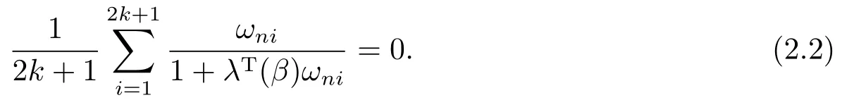
whereλ(β)∈Rris determined by

Theorem 2.1Suppose that Assumptions(A1)and(A2)are satisfied.Then,asn →∞,

whereis a chi-squared distribution random variable withrdegrees of freedom.

Letzα,rsatisfy≤zα,r)=1-αfor 0＜α ＜1.It follows from Theorem 2.1 that an EL-based confidence region forβwith asymptotically correct coverage probability 1-αcan be constructed as

3.Simulation Results

We denote the EL-based confidence region forβgiven by (2.3) as ELCI.On the other hand, from Lemmas 4.4 and 4.5 in Section 4, the confidence region forβbased on the normal approximation as NACI is given by

where

andzα,rsatisfiesP≤zα,r)=1-αfor 0＜α ＜1.

In the simulation, the linear model was taken as:

whereβ=1.5,thewere generated from the uniform distributionU[0,1] with a given seed so that they remained fixed in the simulation, and thewere generated from a AR model below:

where{εt0}is an i.i.d.N(0,1)random variable sequence.We can see that errorεiisα-mixing.

We generated 1,000 random samples of data{(xi,yi),i=1,2,···,n}forn=100,200,300,400 and 500 from Model (3.1).Takep= [n6/25] andq= [n5/25], which satisfy the conditions of Theorem 2.1.For nominal confidence level 1-α= 0.95, using the simulated samples, we evaluated the coverage probabilities (CP) and average lengthes (AL) of ELCI and NACI forβ, which were reported in Tab.1.

Tab.1 Coverage probabilities (CP) and average lengthes (AL) of confidence intervals for β

It can be seen from the simulation results that the coverage probabilities are close to the nominal level and the lengths of the estimated confidence intervals decrease when the sample size increases.In addition, ELCI performs better than NACI since ELCI has higher coverage accuracy and shorter average length than those of NACI.

4.Proofs

We useCto denote a positive conatant independent ofn, which may take a different value for each appearance.To prove our main results, we need following lemmas.

Ifξandηare bounded random variables, then

|E(ξη)-E(ξ)E(η)|≤Cα(m),

whereCis a positive constant.

ProofSee Lemma 1.1 in [18].Note that(4.1)is also true for complex random variables{ξi,1 ≤i≤n}with|a|replaced by the norm of a complex numbera.

Lemma 4.3[19]Let 2＜p0＜r0＜∞and{ηi,i ≥1}be aα-mixing process with E(ηi) = 0 and E|ηi|r0＜∞fori ≥1.Suppose thatα(n) ≤Cn-θfor someC ＞0 andθ ＞p0r0/{2(r0-p0)}.Then,

(4.3) follows if we can show that

As a preparation, we first show that

where we have used Lemma 4.1 withp0=q0=4+δ.

It follows that

From stationarity and Lemma 3.2 in [20], we have

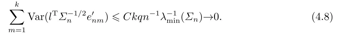
From Lemma 4.1 withp0=q0=4+δ, it can be shown that

(4.8) and (4.9) imply that

Similarly,

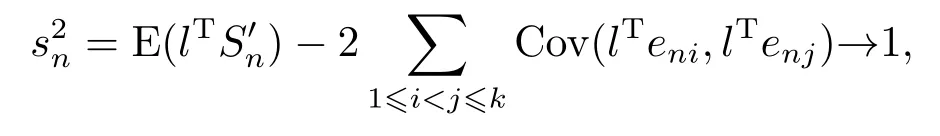
Consequently, we have (4.5) and (4.6).Note that Var(lTSn) = 1 andlTSn=+It follows that

From stationarity and Lemma 3.2 in [20], we have

From Lemma 4.1 withp0=q0=4+δ, we have

It follows from (4.12) and (4.13) that

which proves (4.7).

We now prove (4.4).From Lemma 4.2 and stationarity, we have

which implies that{lT1 ≤m≤k}are asymptotically independent.

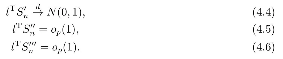
Suppose that{ηnm,1 ≤m≤k}are independent random variables, and the distribution ofηnmis the same as that oflTenmform= 1,2,···,k.By Lemma 4.3 withp0= 3 andr0=4+δ, we have

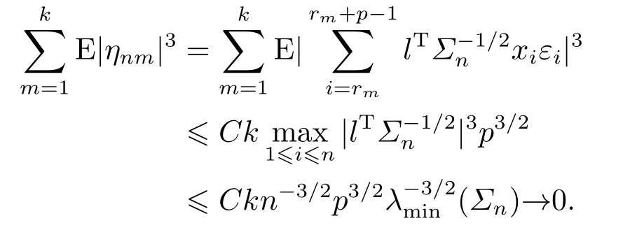
Applying Berry-Esseen’s theorem and1, we get

Thus (4.4) is proved.

From (4.4)-(4.6) and the Cramer-Wold theorem, we obtain Lemma 4.4.

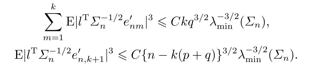
Lemma 4.5Suppose that Assumptions (A1) and (A2) are satisfied.Then, asn →∞,

ProofFromq ≤Cp,n-k(p+q)≤Cpand Lemma 4.1, we have (4.15).(4.16) comes from Lemma 4.4.So we only need to prove (4.17) and (4.18) in the following.

We first prove (4.17).Note that

where

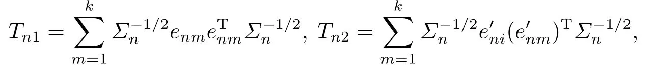
and

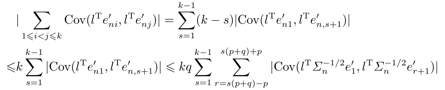
For anyl ∈Rrwith‖l‖=1, from the proof of Lemma 4.4, we can see that

On the other hand, for a given 0＜δ1＜δ/2,we will show that

Takep0=2+δ1andr0=2+δ1+δ2, whereδ2=(2+δ1)(δ-2δ1)/{2(6+δ1+δ)}.From this choice ofδ2, we have

which is a critical observation to use Lemma 4.3 in proving(4.20).From Lemma 4.3, we have

Therefore (4.20) follows.

From the proof of Lemma 4.4, we know E(Tnj) =o(1),j= 2,3, soTnj=op(1),j= 2,3.(4.19) and (4.20) imply (4.17).

We now prove (4.18).It suffices to show, for anyl ∈Rrwith‖l‖=1, that

From Lemma 4.3 withp0=3 andr0=4+δ, we have

Similarly

We thus have (4.21) and (4.18).The proof of Lemma 4.5 is completed.

Proof of Theorem 2.1Letρ=‖λ‖=‖λ(β)‖,λ=λ(β)=ρη.

From(2.2), we have

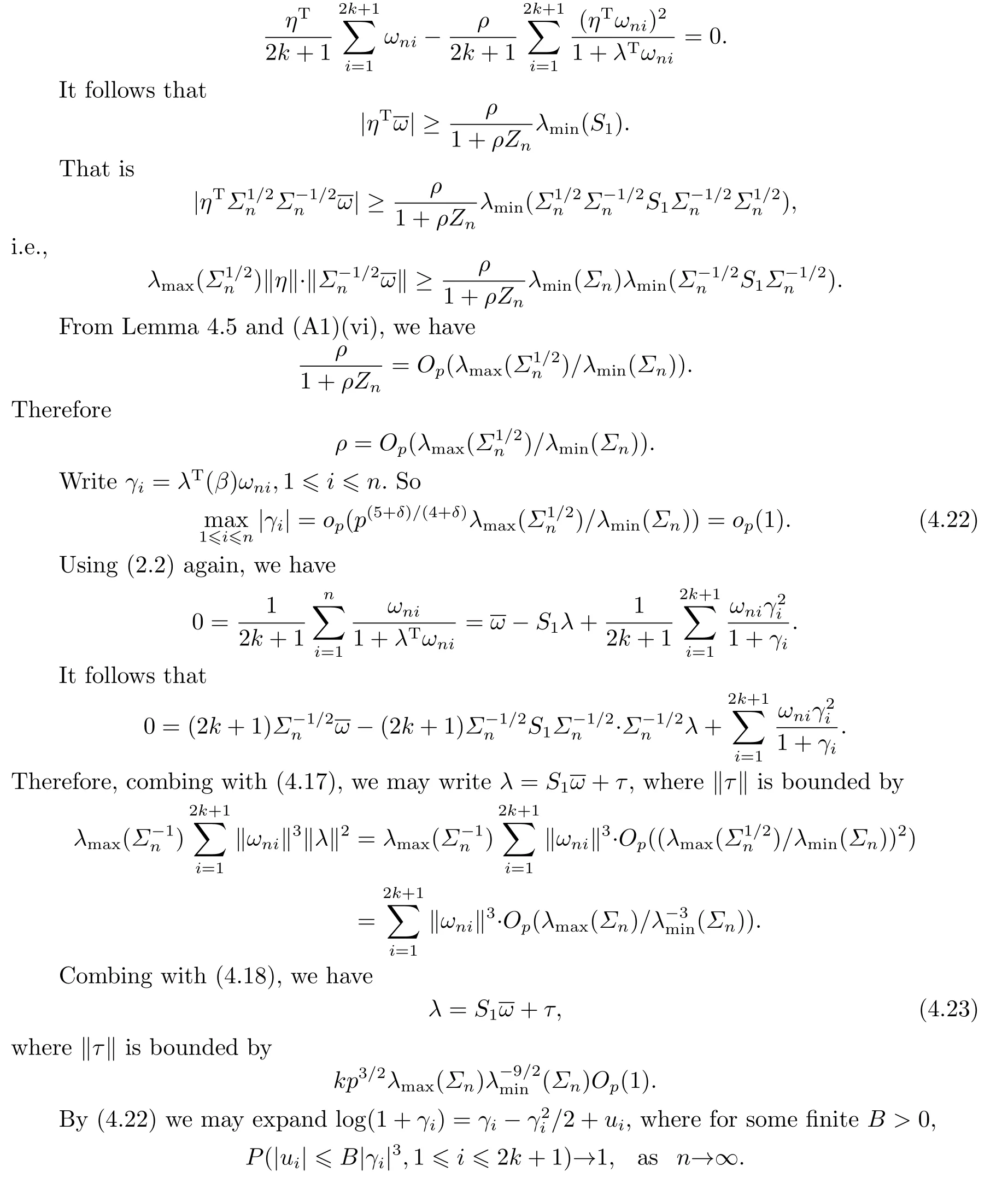
Therefore, from (2.2) and the Taylor expansion, we have

From (4.16) and (4.17), we have

On the other hand

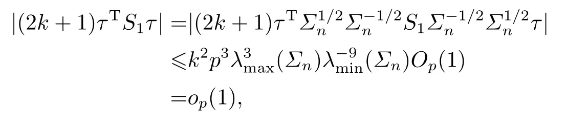
and

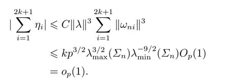
Thus the proof of Theorem 2.1 is completed.