VERA VILLAGRAN Octavio Paulo ∗

Mathematics Department,University of Tarapaca,Arica-Chile.

Abstract. In the present paper we study the well-posedness using the Galerkin method and the stabilization considering multiplier techniques for a fourth-order nonlinear Schr¨odinger equation in domains with moving boundaries. We consider two situations for the stabilization: the conservative case and the dissipative case.

Key Words: Nonlinear Schr¨odinger equation;moving boundary;stabilization.

1 Introduction

In this work we study the existence of the weak solution as well as the asymptotic behaviour of the fourth-order nonlinear Schr¨odinger equation in a bounded domain with moving boundary. Indeed,we consider the following initial value problem

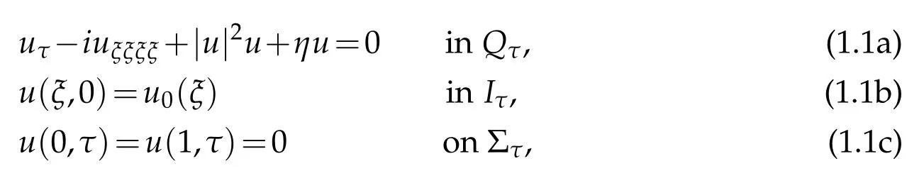
andIτis the time dependent interval given by

whereα(·),β(·)∈C2[0,+∞)are such that

The lateral boundary ΣτofQτis given by

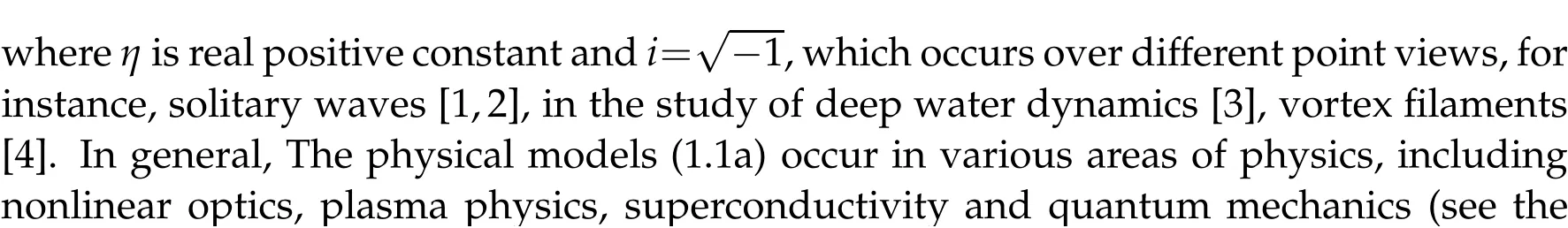
There are many results for the fourth order nonlinear Schr¨odinger equation(see[1,2,6–8]and references cited therein). Especially, the one dimensional case is well studied. The objectives of this work are twofold. To show the existence and uniqueness of the solution to the moving boundary problem(1.1a)and to transform the problem into another initial boundary value problem defined over a cylindrical domain whose sections are not timedependent.We can to note that the solvability and stability of several evolutions models using this strategy have previously been considered[9–12].

The main result of this paper are the following theorems

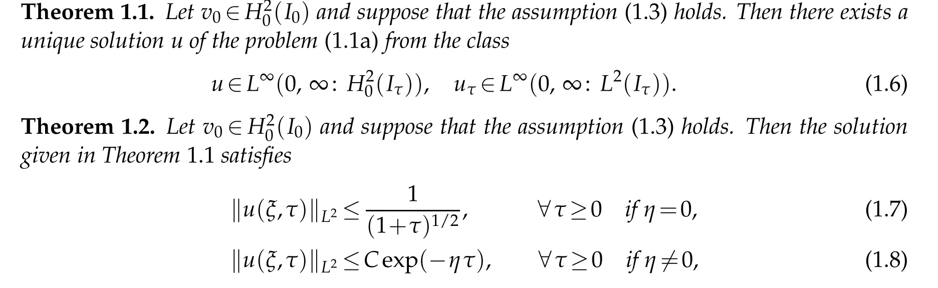
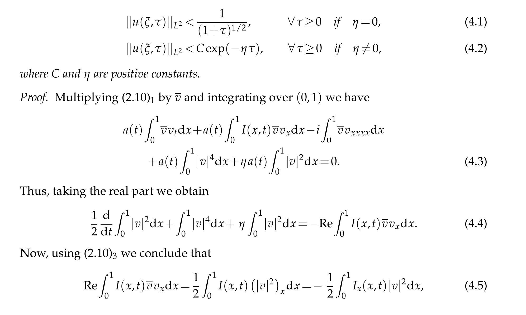
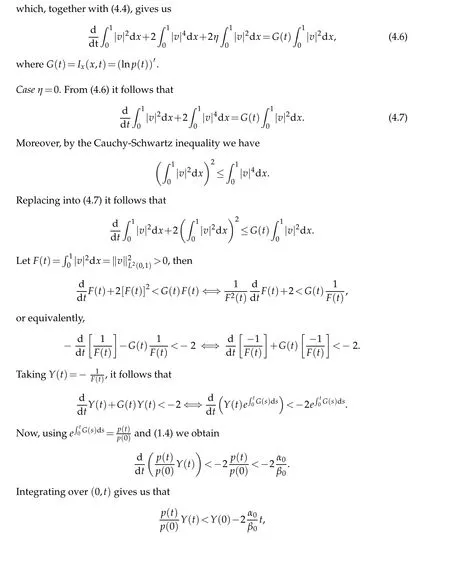
where C and η are positive constants.

Our paper is organized as follows: In Section 2 we transform the moving boundary domain into the cylindrical one. In Section 3 we obtain the existence and uniqueness of solutions to the model. Finally, in Section 4 we analyze the solution of(1.1a)using suitable multiplier techniques.

Finally, throughout this paperCis a generic constant, not necessarily the same at each occasion (it will change from line to line), which depends in an increasing way on the indicated quantities.

2 Transform moving boundary

In this section we will consider a change of variables to transform the time dependent domainQτinto a cylindrical one. The transformation of a moving boundary to a fixed boundary has employed elsewhere[13]. To this end,we consider the application

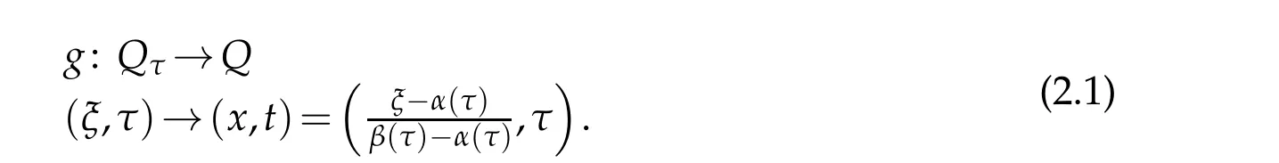
Note thatg∈C2and its inverseg−1is given by

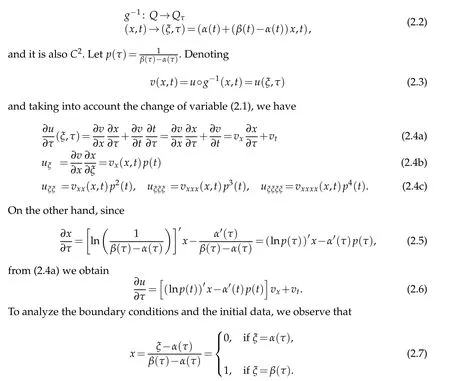
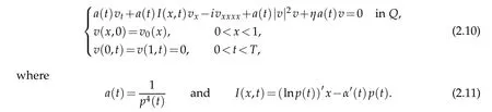
Thus,from(1.1b)–(1.1c)and(2.3)it follows that

v(x,0)=u◦g−1(x,0)=u(α(0)+(β(0)−α(0))x,0)=u0((β(0)−α(0))x+α(0))(2.8)

and Finally,denotingQ=(0,1)×(0,T),v0(x)=u0((β(0)−α(0))x+α(0))and replacing(2.4a)-(2.9)into(1.1a)we obtain the following initial value problem

The following results are going to be used several times in the rest of this paper.

Lemma 2.1. (The Gagliardo-Nirenberg inequality, see [14]). Let q,r be any real numbers satisfying1≤q,r≤∞and let j and m be nonnegative integers such that j≤m.Then

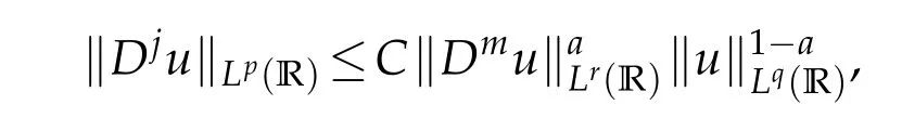
where1/p=j+a((1/r)−m)+(1−a)/q for all a in the interval j/m≤a≤1,and C is a positive constant depending only on m,j,q,r and a.

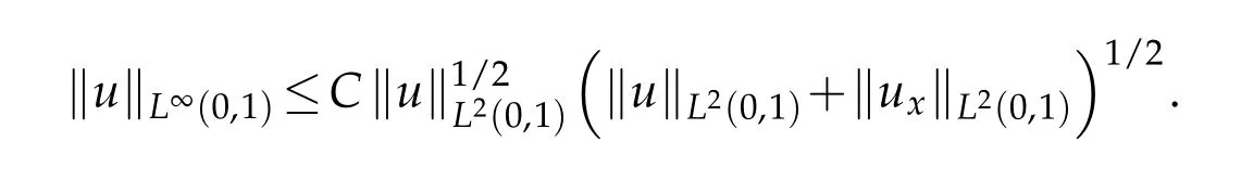
Lemma 2.2. ([12]). For all u∈H1(0,1)it is valid that

3 Well posedness

such that the set of linear combinations of {wn}n∈Nis dense in D(B). Let us denote byVmthe space generated by[w1,...,wm],so that we may construct approximations

forj=1,...,m. Using classical theory of ordinary differential equations, we can prove that the system(3.3)-(3.4)has a local solution in the interval(0,tm)(see[15]). To show the existence of solutions in the interval(0,T)independent ofm,we need a priori estimates.

Remark 1. We are employing the standards notation(·,·)for theL2(0,1)inner product.

3.1 A priori estimates

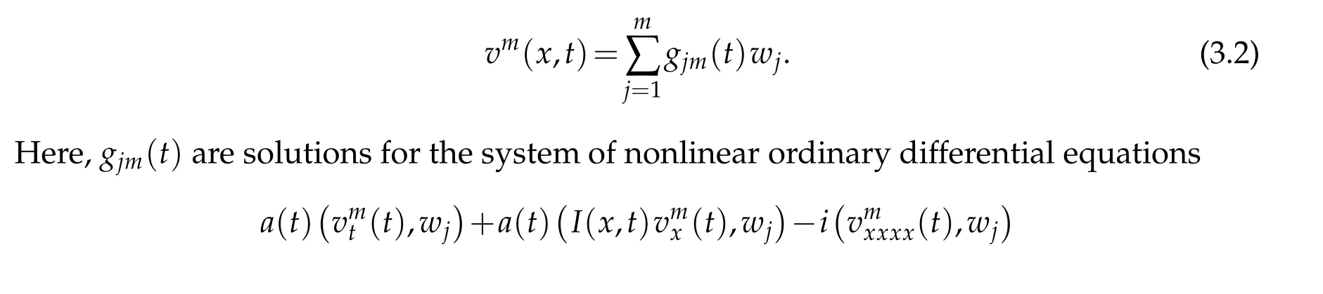
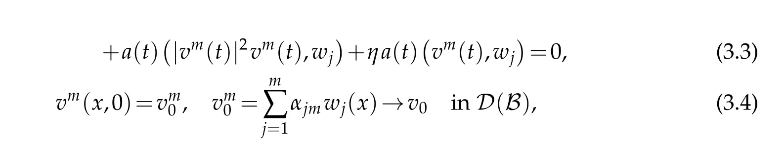
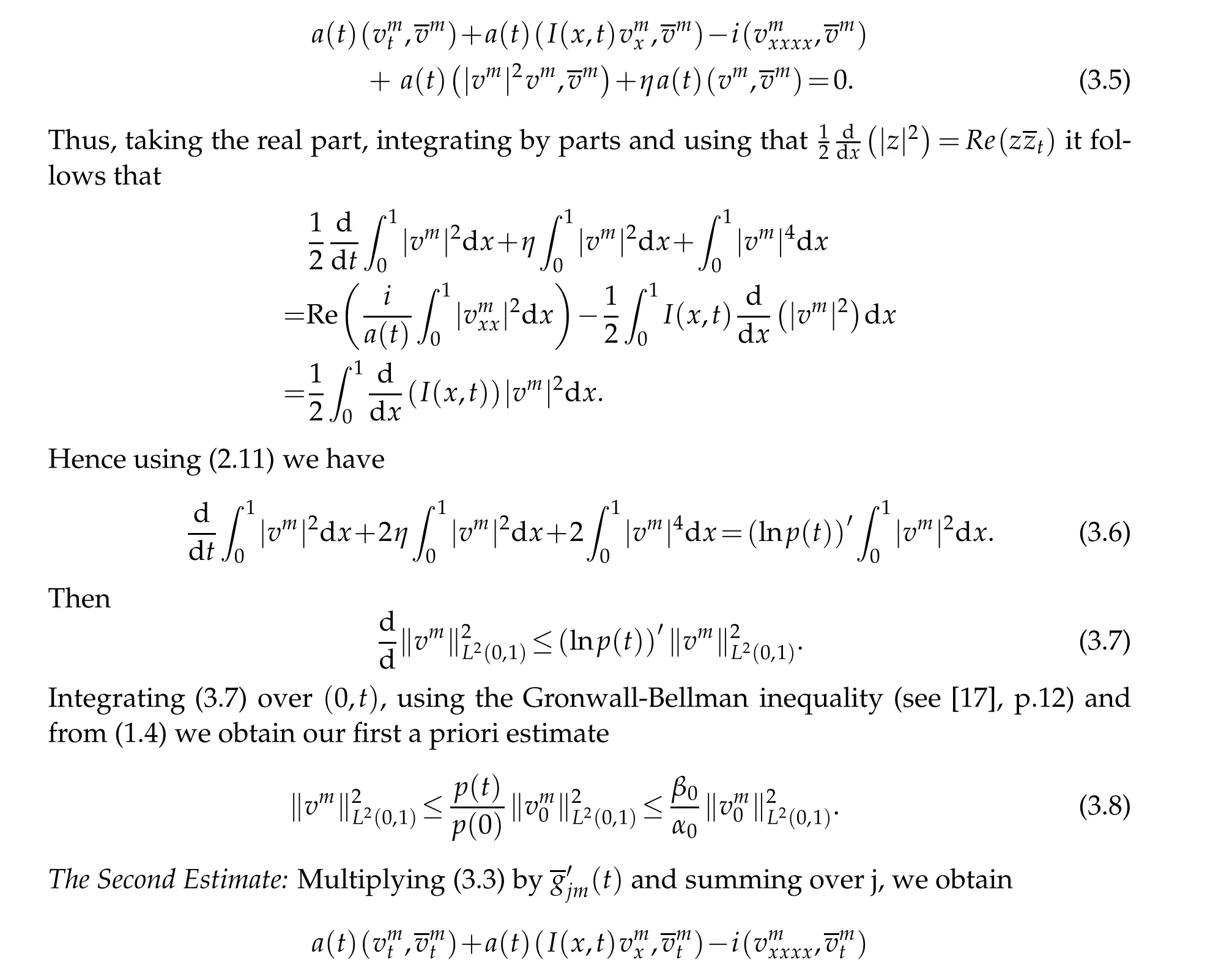
The First Estimate:Multiplying equation (3.3) bygjm(t) and summing up the product result over j,we have

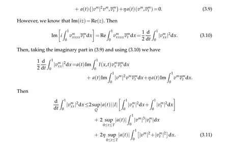
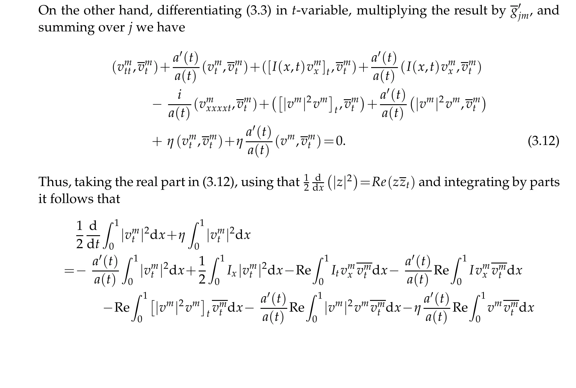
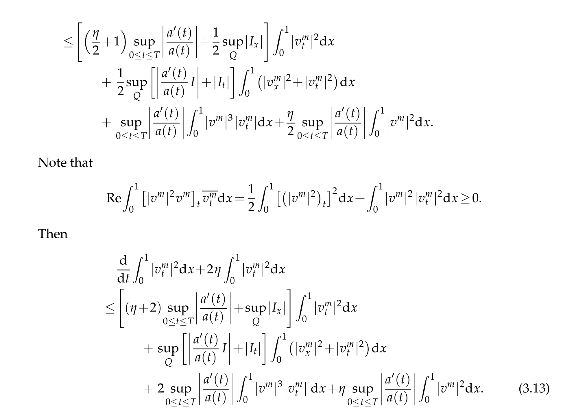
Adding(3.11)and(3.13)we obtain

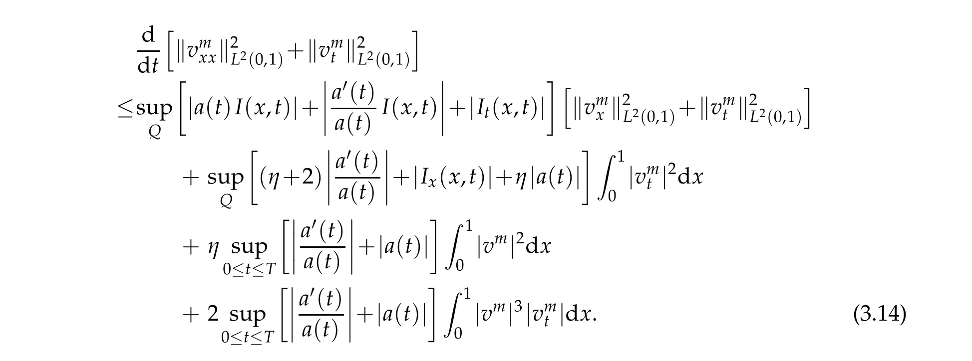
Therefore,thanks to assumptions onα(t)andβ(t),we arrive at

Hence,

3.2 Existence and uniqueness of solutions of(2.10)

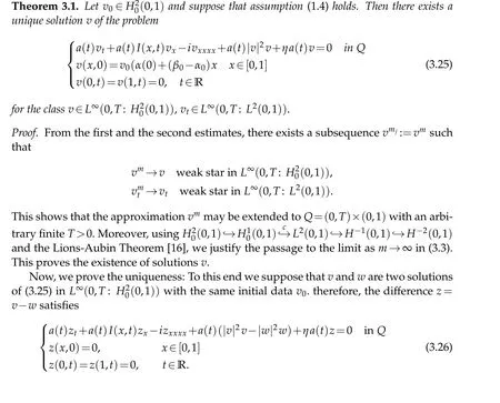
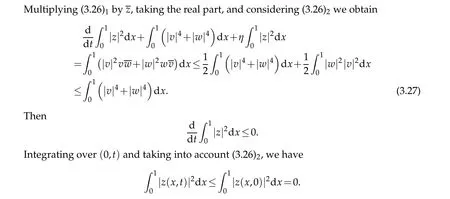
Thusz=0,and the uniqueness follows.

4 Stability

Theorem 4.1.Let u0∈H20(Iτ)and suppose that the assumption(1.4)holds. Then the solution of(1.1a)given by Theorem3.1satisfies

Acknowledgement

The author is partially financed by regular project Fondecyt 1191137. ANID.Chile.