MA Rui, XIONG Xiangtuan,∗and AMIN Mohammed Elmustafa,2

1 Department of Mathematics,Northwest Normal University,China.

2 Department of Mathematics,Omdurman Islamic University,Khartoum,Sudan.

Abstract. We consider an inverse heat conduction problem with variable coefficient on an annulus domain. In many practice applications, we cannot know the initial temperature during heat process, therefore we consider a non-characteristic Cauchy problem for the heat equation. The method of fundamental solutions is applied to solve this problem.Due to ill-posedness of this problem,we first discretize the problem and then regularize it in the form of discrete equation. Numerical tests are conducted for showing the effectiveness of the proposed method.

Key Words: Inverse heat conduction problem; method of fundamental solutions (MFS);Cauchy problem;Ill-posed problem.

1 Introduction

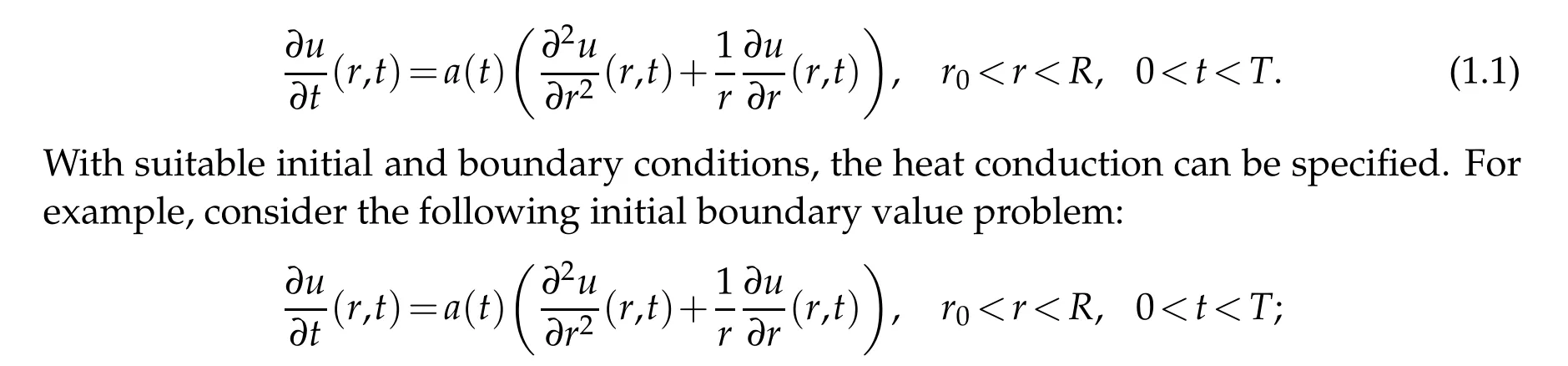
In the process of heat conduction on an annulus domain, the following heat equation with variable coefficient is a good mathematical model in many situations:

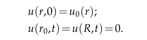
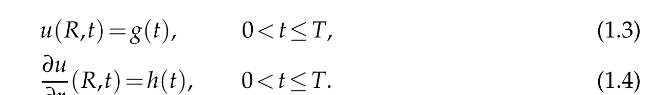
If the suitable regularity of the datau0(r)and the coefficienta(t)is given,one can prove the well-poseness of the classical problem for the solutionu. Generally,we call it the direct problem.But in many engineering problems,the initial condition cannot be obtained because one cannot know when the heat conduction begins. Usually we want to know the temperature on inaccessible interior boundary of a pipe,but only the measurements from the outer boundary are available, this can be formulated as an inverse problems witha(t)>0:

with Dirichlet and Neumann data on the known boundaryR(accessible for data measurement)

In this paper,we want to recover the initial temperatureu(r,0)and the inner boundary temperatureu(r0=0,t).This inverse heat conduction problem is called non-characteristic Cauchy problem mathematically. It is a well-known severely ill-posed problems. For illposed problems of mathematics physical equations,there are two ways to deal with. the first way is to discretize the problem first and then regularize it. The other way is to regularize it first and then discretize it. For example, for the fist way we can use the finite difference method to discretize the PDE-model problem and then an ill-posed discritized system is obtained and one can use all kinds of regularization methods[1,2](e.g.truncated singular value decomposition)to treat it. For the second way,we make the ill-posed PDE-model problem to be well-posed,and then one can use all kinds of numerical methods for solving the well-posed problem. In this paper, we use the first way. To do that,we use the MFS to discretize the problem,and then we use the Tikhonov method to regularize it. As in[3],we emphasize the advantages of the MFS:“it is simple and feasible to handle various boundary conditions;it is easier to solve inverse problems than boundary element method, finite element method and finite difference method; it is applicable to solve more complex problems.”

The MFS is a meshless method. It is first used to solve inverse heat conduction problem in [4] and then it is extended to solve all kinds of inverse problems [5-13]. It has been proved that the MFS with regularization methods is an efficient method for solving inverse and ill-posed problems.

A problem which is similar to(1.2)-(1.4) has been considered in[3]. But the problem in[3]is considered in the Cartesian coordinates.The fundamental solutions in this paper are more complex and it cause the computation is more difficult. In addition,we choose the source points in the way that is very different from the literature [3]. Numerical results show that our method is more stable. We believe that our method can be attracted more theoretical research.

The outline of this paper is as follows. In Sec. 2, we present the formulation of the inverse problem and give the MFS to solve the inverse problem,in Sec.3 some numerical experiments are tested.

2 Model problem and MFS

The inverse heat conduction problem on an annulus is mathematically described by the following governing equation

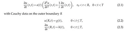
without loss of the physical meaning,we can assume thata(t)>0.

In this paper,our interest is to reconstruct the temperature datau(r0,t)and the initial datau(r,0)from the Cauchy data pairs(g(t),h(t)).

The MFS is conducted as follows. First the fundamental solution of the governing of Eq.(2.1)can be obtained using a simple transformation.

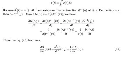
Let The fundamental solution of Eq. (2.4)is

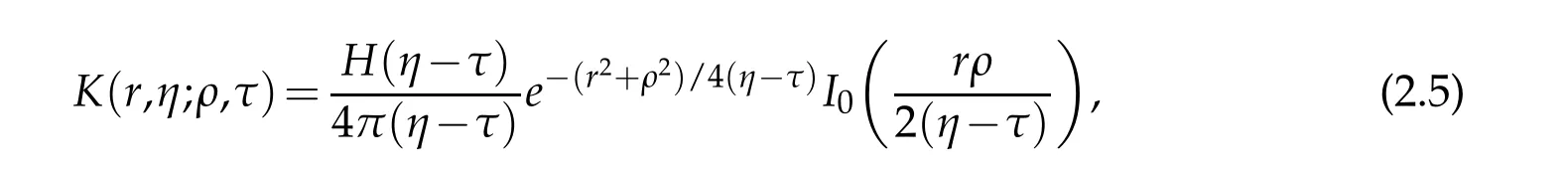
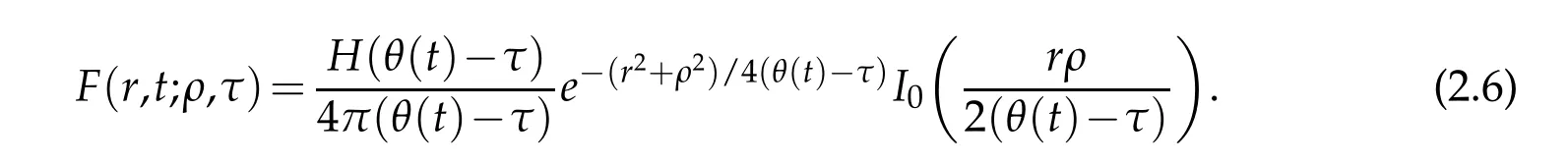
whereHis the Heaviside function andI0is the modified Bessel function of the first kind of order zero. From above the fundamental solution of original Eq. (2.1)can be given by

Usually, the Dirichlet and Neumann boundary conditions (2.2) and (2.3) are measured only at some discrete points with random noises. Assume that the data are collected at the pointsti,i=1,...,Mon {R}×[0,T] satisfying the Dirichlet and Neumann boundary conditions(2.2)and(2.3)respectively,and we have:

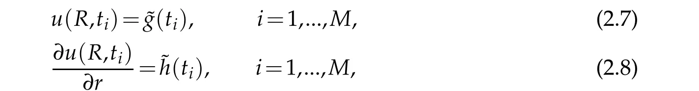
where ˜g(ti)and ˜h(ti)are randomly perturbed data(Gaussian distributed random vector)of the functionsgandhwith a noise levelδ>0.

We generate an approximation to the radial heat equation(2.1)by using a linear combination of fundamental solutions given by

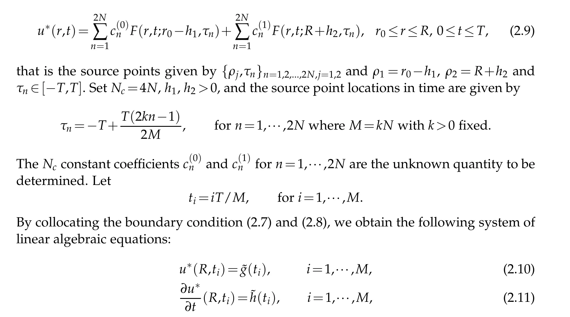
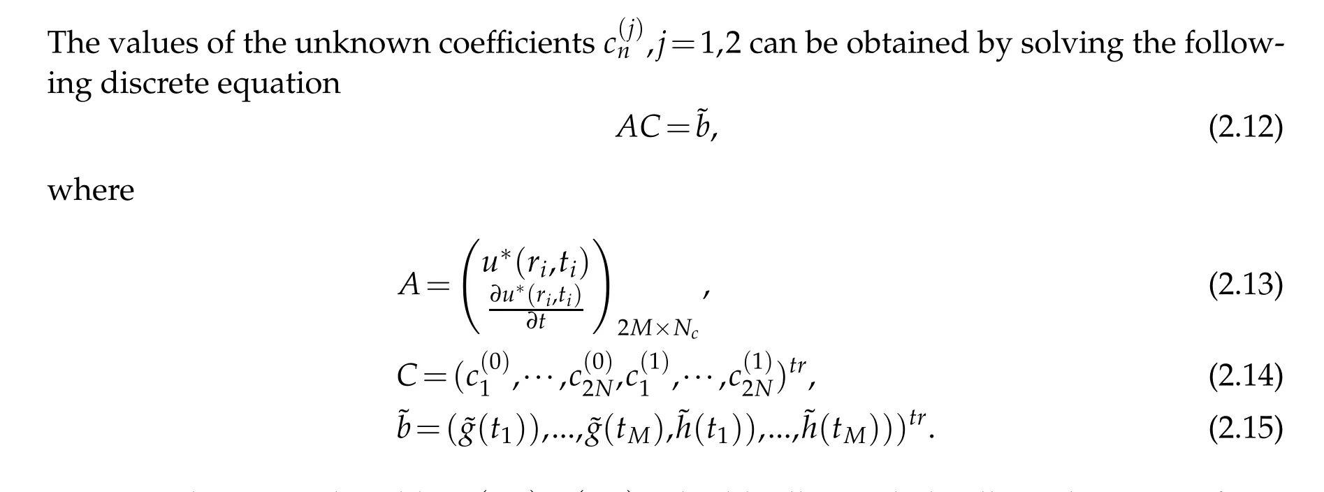
Since the original problem(2.1)−(2.3)is highly ill-posed,the ill-conditioning of matrixAin Eq.(2.12)still exists.That is to say that most classical numerical methods cannot applied for solving the matrix Eq. (2.12) because the problem is ill-posed and unstable.Many regularization methods have been developed for solving these kinds of discrete ill-posed problems. In our numerical experiments,we use the classical Tikhonov regularization to solve the Eq. (2.12). The Tikhonov regularized solution for Eq. (2.12)is defined to be the solution to the following least-squares problem:

where‖·‖denotes the usual Euclidean norm andαis the regularization parameter.

The identification of the regularization parameter is very important for the quality of the regularization solution. In our test we use the well-known L-curve method which is a kind of noise-free rules, to determine the regularization parameterα. In numerical computation,we used the Matlab code developed by Hansen[14,15]for solving the discrete ill-conditioned system(2.12). Define the Tikhonov regularization solution of(2.12)byCα∗. The approximated solutionuα∗for problem(2.1)-(2.3)is then given by

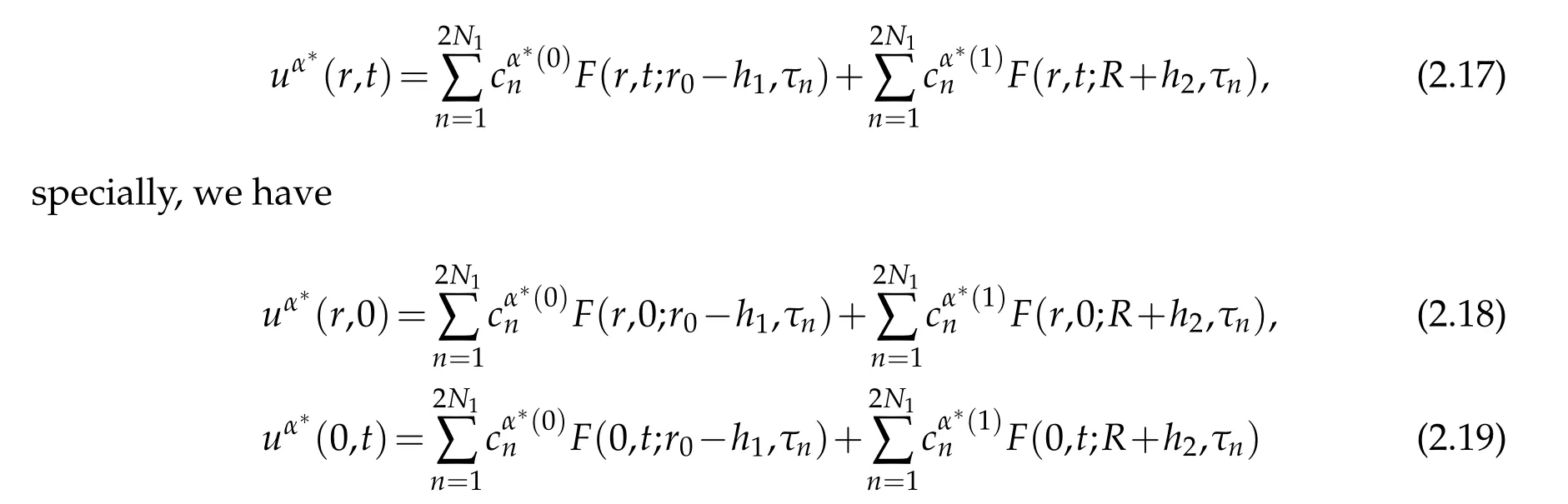
as the numerical solution of(2.1)-(2.3).

3 Numerical tests

To demonstrate the effectiveness and stability of the proposed numerical method in this section, we present three examples. And we use the root mean square error (RMS) to measure the accuracy of the approximate solutions tou(r,0),u(0,t):

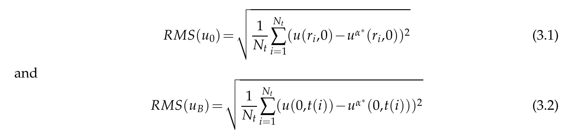
whereNtis the total number of testing points, andu,uα∗are respectively the exact and approximated value.In these examples,we add random noise to the data as the following way: ˜g=g+δ∗rand(size(g)), ˜h=h+δ∗rand(size(g)), and we always chooseM=40,Nc=80.

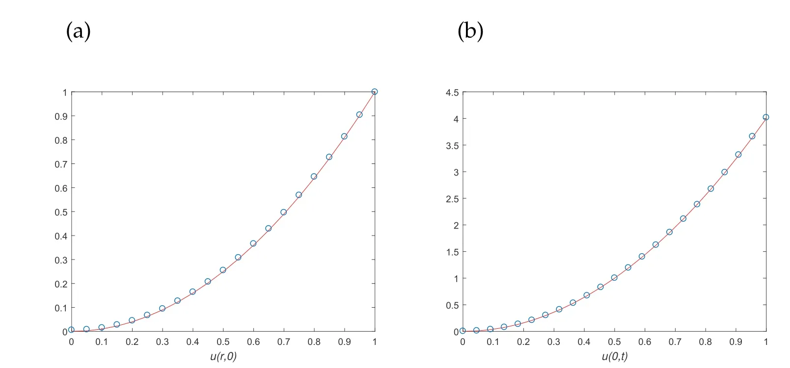
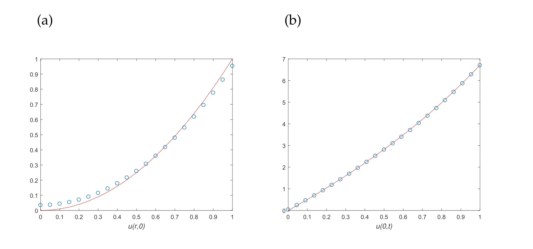
Example 3.1. The exact solution of the problem(2.1)-(2.3)is given by:

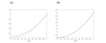
In this example, we chooseT=1 andh1=h2=2 and the noise levelδequals to 0.01 and 0.05 in Figs. 1 and 2 respectively. The numerical result of the proposed method is presented in Figs. 1 and 2. Figure 1(a) shows the exact solution and numerical solution at the initial time. The RMS of the initial temperature isRMS(u0) =0.0049. Figure 1(b)shows the exact solution and numerical solution at the inner boundary {r0=0}×[0,T].The RMS of the inner boundary temperature isRMS(uB)=0.0067. We can see that the numerical method works well for the initial temperature and inner boundary temperature. In Fig. 2,the numerical results with a larger noise levelδ=0.05 are presented. It is easy to see that the method performs very well,too.

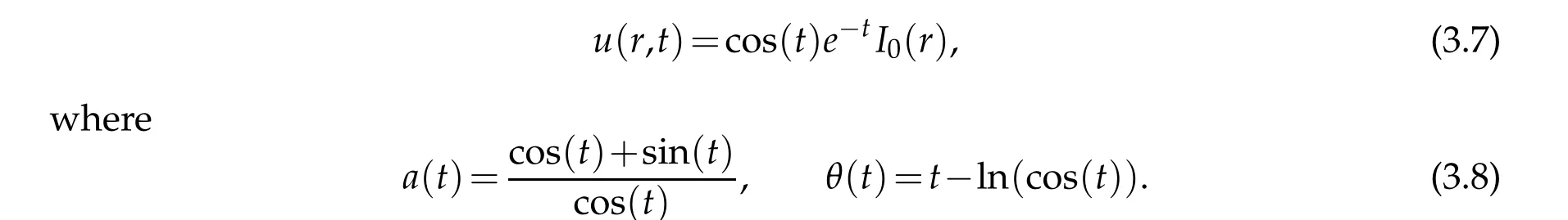
Example 3.2. The exact solution is given by

In this test,we chooseT=1 andh1=h2=3 andδ=0.01,α∗=6.6×10−5andδ=0.05,α∗=1.2×10−4in Figs.3 and 4 respectively.The results of the proposed method are presented in Figs. 3 and 4.

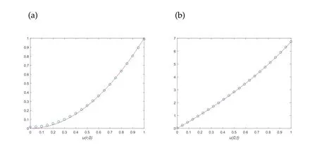
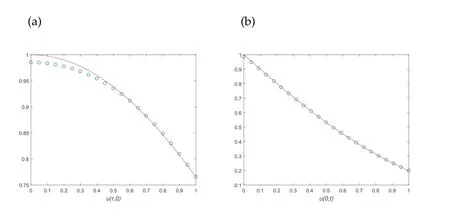
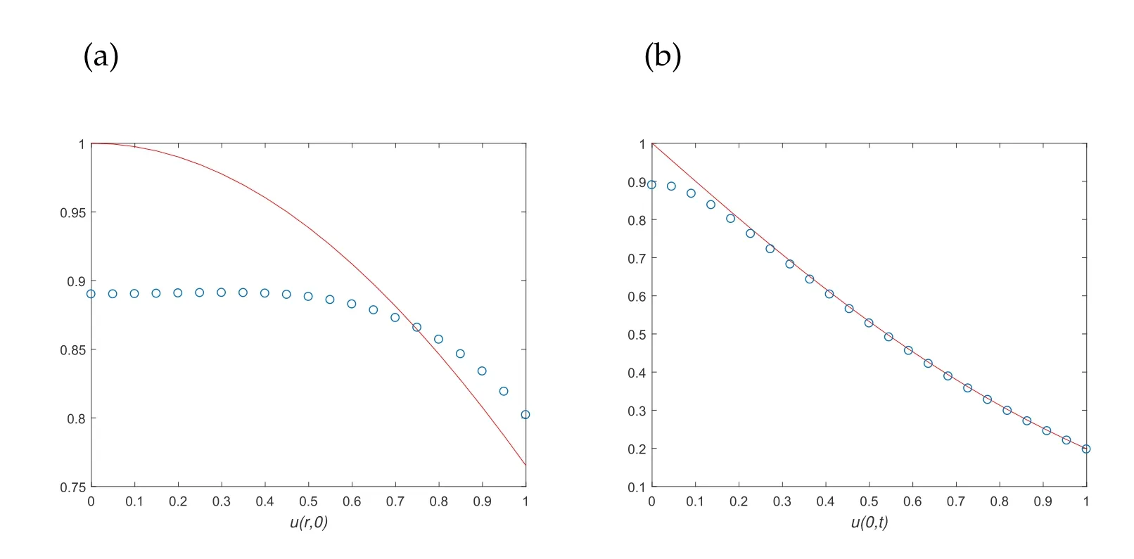
Example 3.3. Here we have the exact solution for the problem:

In this example, we chooseT=1 andh1=h2=3 andδ=0.01,α∗=2.8×10−5andδ=0.05,α∗=5.2×10−4in Figs.5 and 6 respectively.And the number of test pointNt=21 in all examples.The results of the proposed method are presented in Figs. 5 and 6.

4 Conclusion

In this paper,we develop the method of fundamental solution for solving a radially symmetric Cauchy problem for heat equation with variable coefficient. Three examples were investigated. Accurate and stable results were obtained. Some open problems(e.g.,the choice of theh1andh2)are still under consideration.

Acknowledgement

We thank the referees for careful reviewing and for pointing out some nice ideas. This research is partially supported by the Natural Science Foundation of Northwest Normal University,China(No. NWNU-LKQN-17-5).