Conditional Regularity of Weak Solutions to the 3D Magnetic B´enard Fluid System
2021-10-23MALiangliang
MA Liangliang
Department of Applied Mathematics,Chengdu University of Technology,Chengdu 610059,China.
Abstract. This paper concerns about the regularity conditions of weak solutions to the magnetic B´enard fluid system in R3.We show that a weak solution(u,b,θ)(·,t)of the 3D magnetic B´enard fluid system defined in[0,T),which satisfies some regularity requirement as(u,b,θ),is regular in R3×(0,T)and can be extended as a C∞solution beyond T.
Key Words:Magnetic B´enard fluid system;regularity criteria;conditional regularity;Morrey-Campanato space;Besov space.
1 Introduction
Consider the unforced magnetic B´enard fluid system for incompressible flows on all space R3:
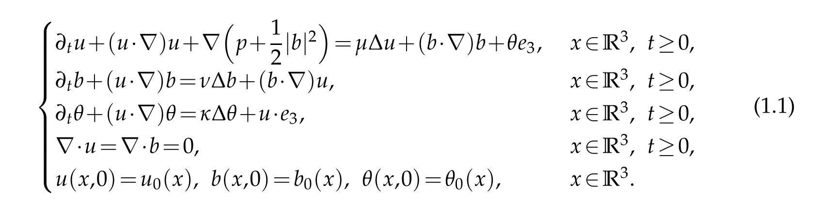
Hereu(x,t)=(u1(x,t),u2(x,t),u3(x,t))∈R3denotes the incompressible velocity field,b(x,t)=(b1(x,t),b2(x,t),b3(x,t))∈R3the magnetic field,θ(x,t)∈R the temperature,p(x,t)∈R the hydrostatic pressure ande3=(0,0,1)the vertical unit vector.The positive constantsµ,νandκare associated with specific properties of the fluid:The constantµis the kinematic viscosity,ν−1is the magnetic Reynolds number andκis the coefficient of thermal diffusivity.The forcing termθe3in the momentum equation describes the acting of the buoyancy force on fluid motion andu·e3models the Rayleigh-B´enard convection in a heated inviscid fluid.The initial data for the velocity and magnetic fields and temperature,is given byu0,b0andθ0in (1.1),and satisfies ∇·u0=∇·b0=0.Finally,(e1,e2,e3)represents the canonical basis of R3.
The equations of thermohydraulics is a couple system a equations of fluid velocity and temperature.Widely known as the B´enard problem,such a system has been under intensive investigation for many decades,in particular concerning its stability (see [1]and Chapter III,Section 3.5 [2]).Furthermore,due to the necessity to consider the behavior of the thermal instability under the influence of the magnetic field,the magnetic B´enard problem has also caught much attention(e.g.[3,4] and also [5] in the stochastic case).The system of equations(1.1)atb≡θ≡0 recovers the Navier-Stokes equations and the system of(1.1) atθ≡0 recovers the magnetohydrodynamics(MHD)system and the system(1.1)atb≡0 recovers the B´enard system.All of those systems have been studied intensively in particular concerning whether given initial data sufficiently smooth,the solution remains smooth or experiences a finite time shock.We recall here,without any claim of completeness,see[7–14]and the references cited therein.
When all three parametersµ,νandκare positive,the global regularity of 2D magnetic B´enard fluid system follows from a standard process.However,it remains a remarkable open problem whether classical solutions of the 2D inviscid magnetic B´enard fluid system,all three parameters are zero,preserve their regularity for all time or finite time blow-up.Whenµ>0,ν>0 andκ=0,the global well-posedness result was proved by Zhou-Nakamura[15].Cheng and Du dealt with the Cauchy problem of the 2D magnetic B´enard fluid system with mixed partial viscosity in [16].They proved the global wellposedness of 2D magnetic B´enard fluid system without thermal diffusivity and with vertical or horizontal magnetic diffusion.Furthermore,they obtained the global regularity and some condition regularity of strong solutions for 2D magnetic B´enard fluid system with mixed partial viscosity.Particularly,the authors in[11]considered the global weak solution of the 2D B´enard system with partial dissipation and established some regularity criteria for the corresponding B´enard system.
It is currently unknown whether the solutions of 3D magnetic B´enard fluid system is globally regular (in time).The author in [17] dealt with the Cauchy problem to the 3D system of incompressible magnetic B´enard fluids,they proved that as the initial data satisfywhereεis a suitably small positive number,the three-dimensional magnetic B´enard system with mixed partial dissipation,magnetic diffusion and thermal diffusivity admit global smooth solutions.Zhang and Tang[18]established the global regularity for a special family of axisymmetric solutions to 3D magnetic B´enard fluid system.
The 2D flow generates a large family of 3D flow with vorticity stretching [19];we refer to these asflows because the flow in thex3direction is predetermined by the underlying 2D flows.Very recently,we studied the global regularity for themagnetic B´enard system with mixed partial viscosity.More precisely,we not only showed the global regularity for themagnetic B´enard system with zero thermal diffusivity by a well-known property of Hardy space and BMO,but also obtained the global regularity for themagnetic B´enard system with zero thermal diffusivity and horizontal magnetic diffusion as well as vertical magnetic diffusion resorting to the method of the local-in-time analysis in[20].
Motivated by the works[21–26],the purpose of this paper is to study the regularity conditions to the magnetic B´enard fluid system(1.1).Our main results in this paper can be stated as follows.
Theorem 1.1.Assume that(u0,b0,θ0)∈L2(R3)with∇·u0=∇·b0=0.Let the triple(u,b,θ)is the weak solution and satisfy the energy inequality of strong form:
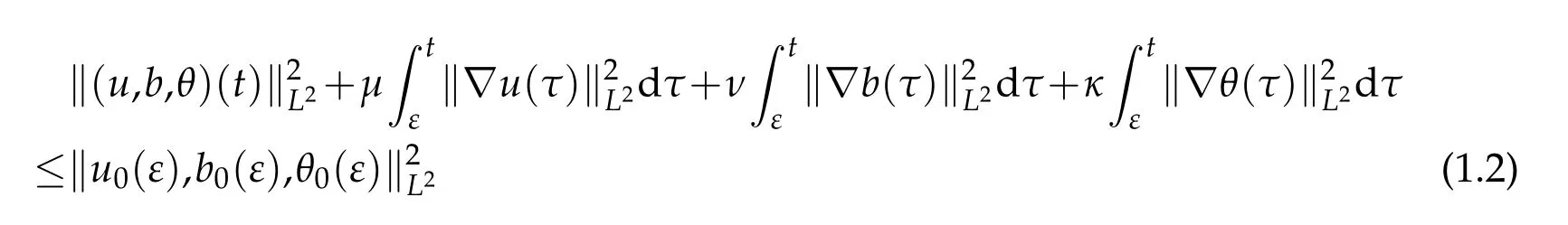
for0≤ε≤t≤T.If one of the following conditions holds
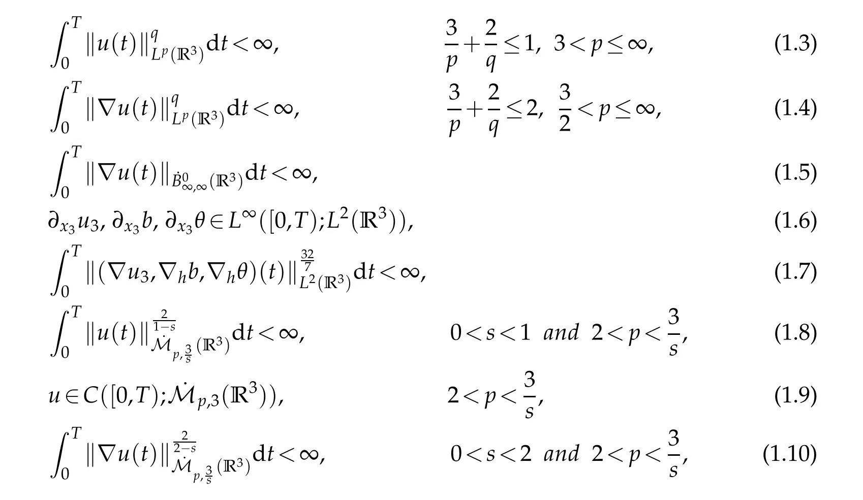
then the triple(u,b,θ)is the smooth solution on[0,T)with the initial value(u0,b0,θ0).
Remark 1.1.The regularity criteria of weak solutions to the magnetic B´enard fluid system (1.1) play an important role to understanding the physical essence of the magnetic B´enard fluid.As it is demonstrated in references[27,28],we also prove that to secure the regularity of weak solutions to system(1.1),one only needs to impose conditions on the velocity field of the fluids.This also demonstrated that in the regularity of weak solutions,the magnetic fieldband the temperatureθof particles play a less important role than the velocityudoes,and the regularity of weak solutions to(1.1)is dominated by the velocityuof the fluids.
Remark 1.2.Sincep=q,the last three conditions in Theorem 1.1 improve the first four conditions in Theorem 1.1.
We conclude this section by describing the plan of this paper.Section 2 describes notations and definitions we have used in this paper,and presents some important lemmas.Section 3 contains the proof of Theorem 1.1.
2 Preludes
This section presents the related notations and definitions as well as lemmas that will be needed for the proofs of the main theorems.
2.1 Notations and definition
1.The vector fields are denoted by
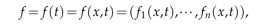
wherex∈R3,t∈[0,T)andn∈N.
2.The gradient field is defined by ∇f=(∇f1,···,∇fn) withf=(f1,···,fn),∇fj=(D1fj,D2fj,D3fj)(j=1,···,n)with
3.The usual Laplacianf=(f1,···,fn)is established by ∆f=(∆f1,···,∆fn),where
4.∇h frepresents the horizontal gradient off,∆h fdenotes the horizontal Laplacian.
5.The standard divergence is given by ∇·f=
6.In the magnetic B´enard fluid system(1.1),the notationf·∇gmeanswheref=(f1,f2,f3)andg=(g1,g2,g3).
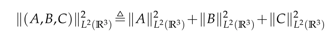
7.Lp(X)denotes the Lebesgue space(1≤p≤∞).Here theLp-norm offis given by
8.Assuming that(X,‖·‖)is a Banach space andT>0,the spaceL∞([0,T];X)contains all measurable functionsf:[0,T]→Xfor which the following norm is finite:
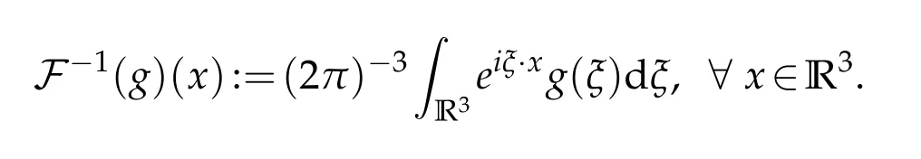
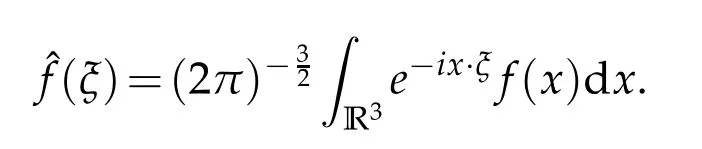
9.Define the Fourier transform offby
whereξ·x=,x=(x1,x2,x3)∈R3,and its inverse by
10.The non-homogeneous Sobolev spaceHs(R3)is
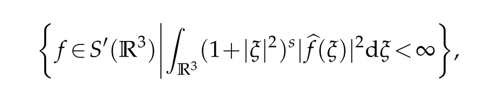
whereS′(R3)is the space of tempered distributions.
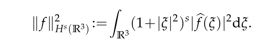
The correspondingHs(R3)-norm is
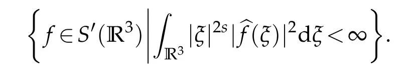
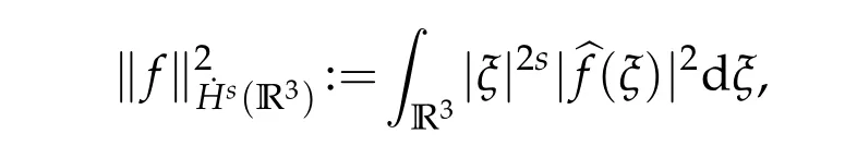
where|x|2=|x1|2+···+|xn|2,withx=(x1,···,xn)∈Cn(n∈N).
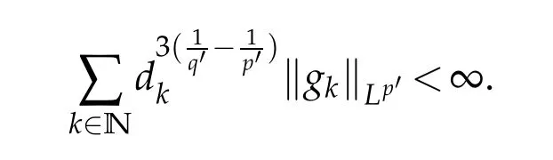
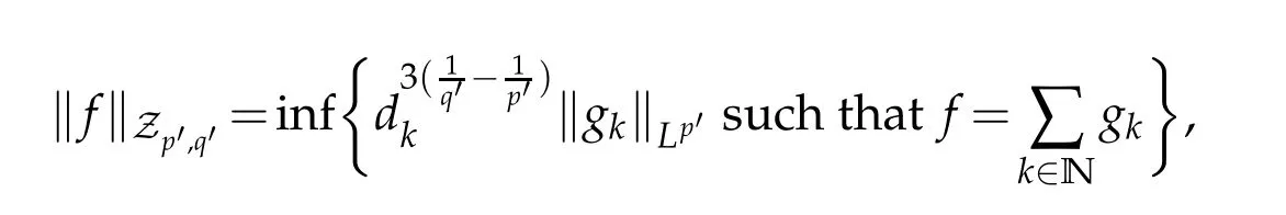
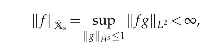
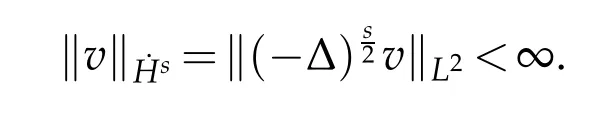
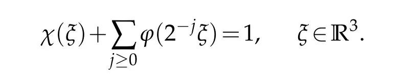
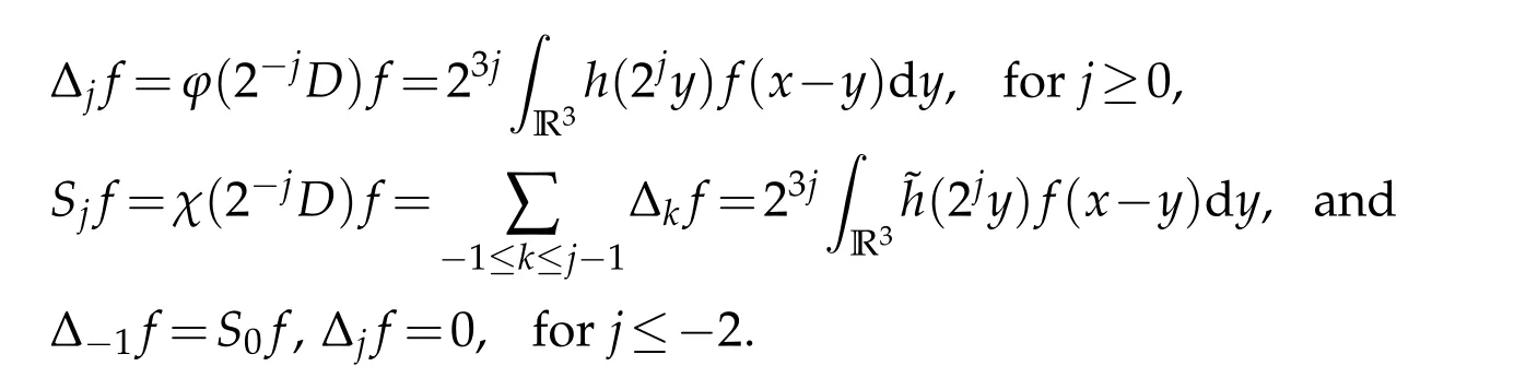
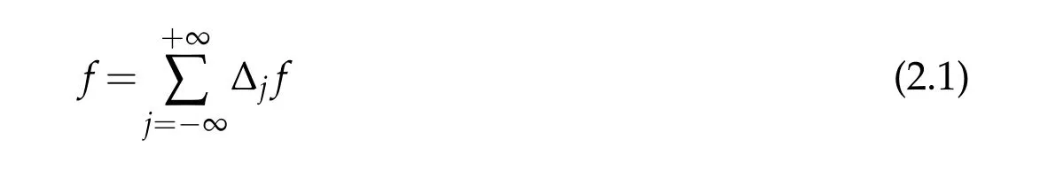
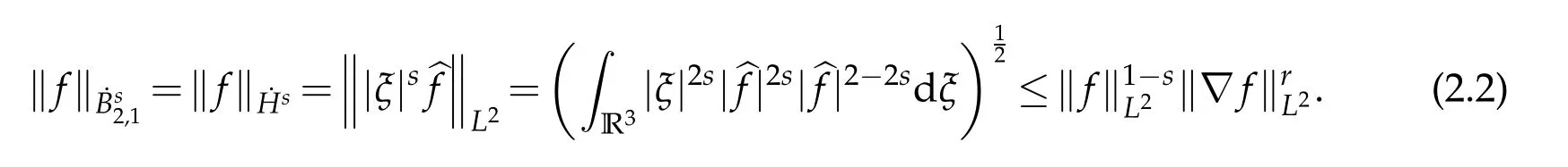
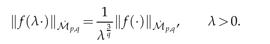
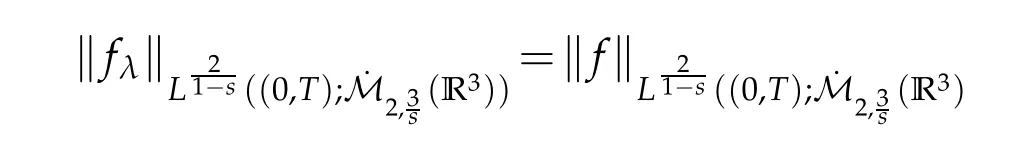
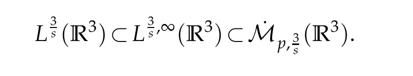
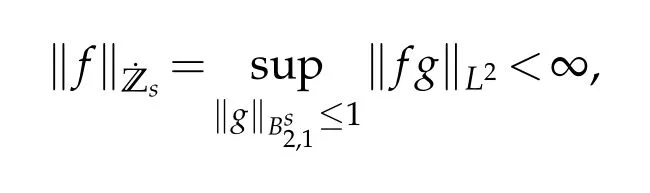
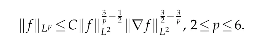
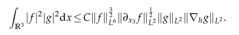
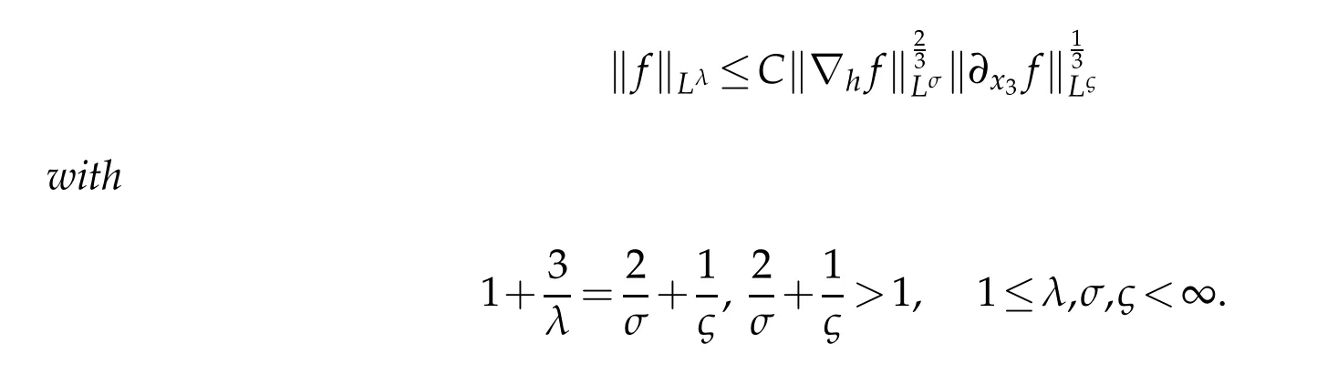
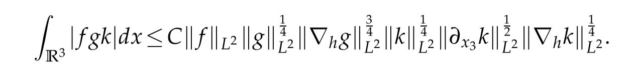
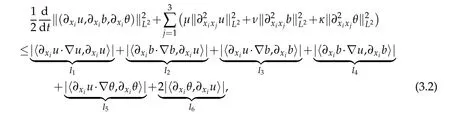
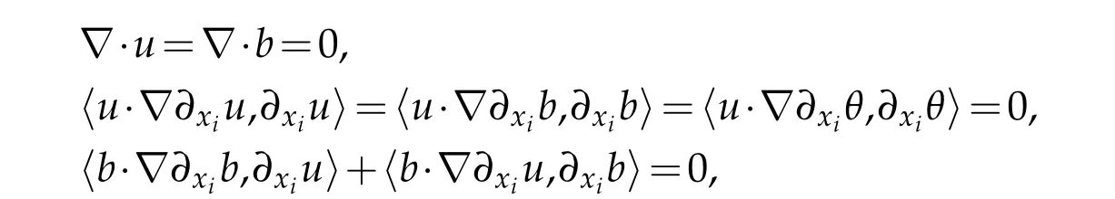
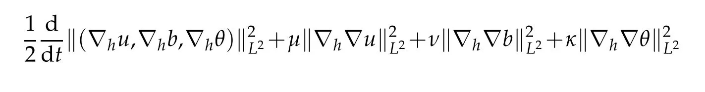
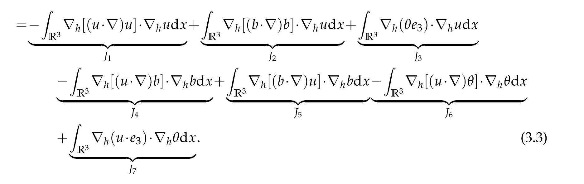
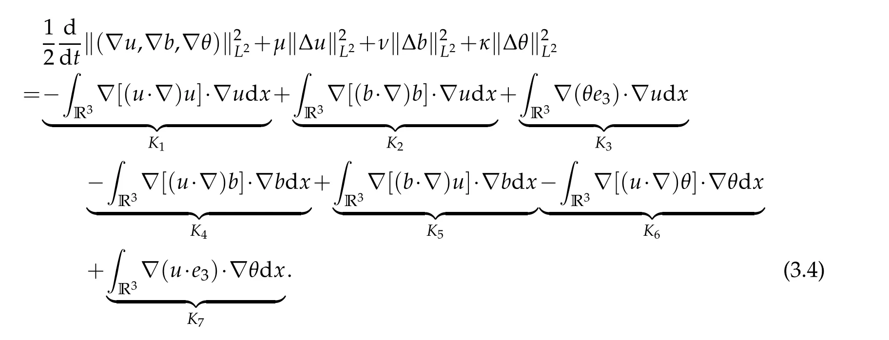
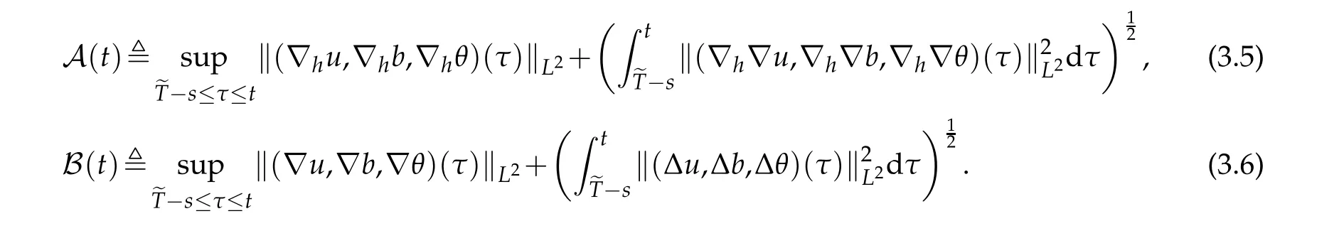
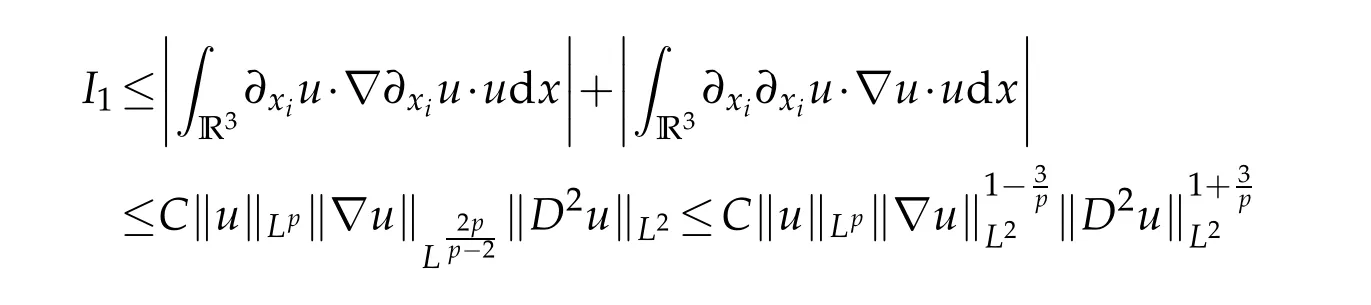
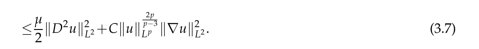
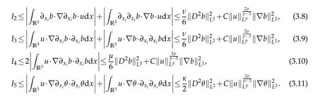
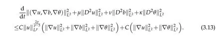
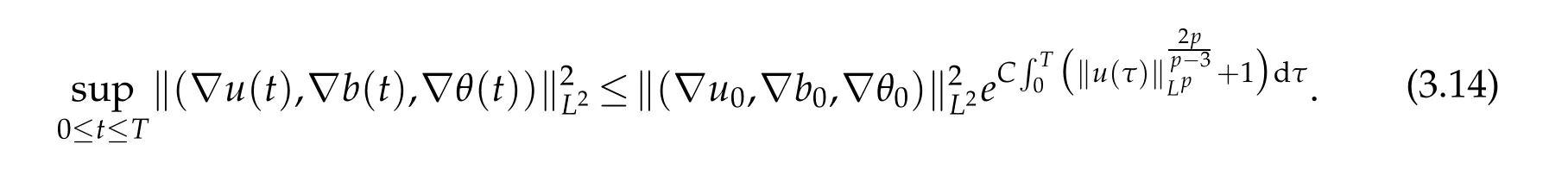
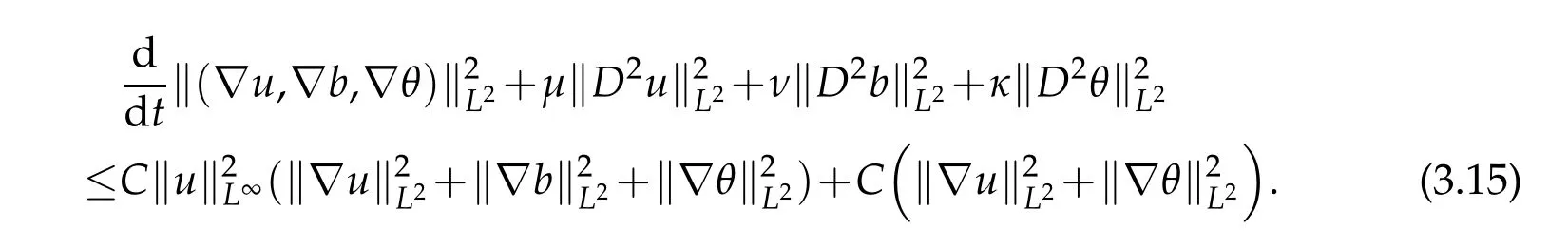
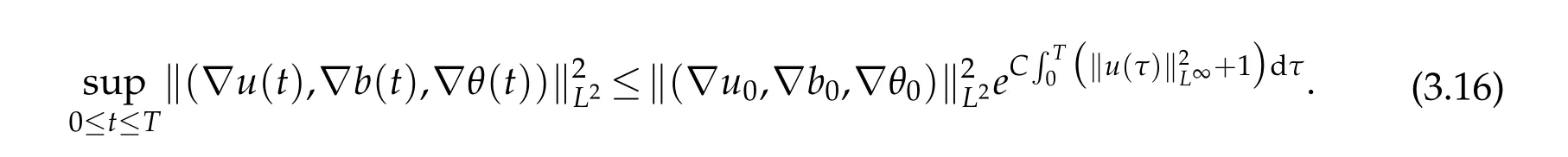
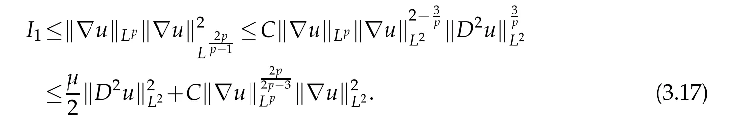
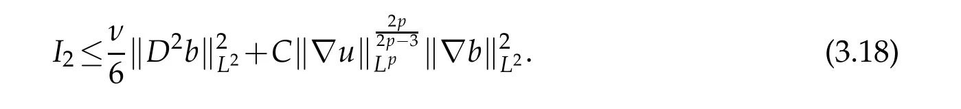
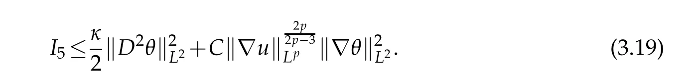
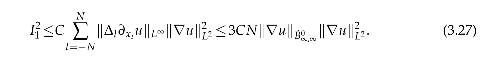
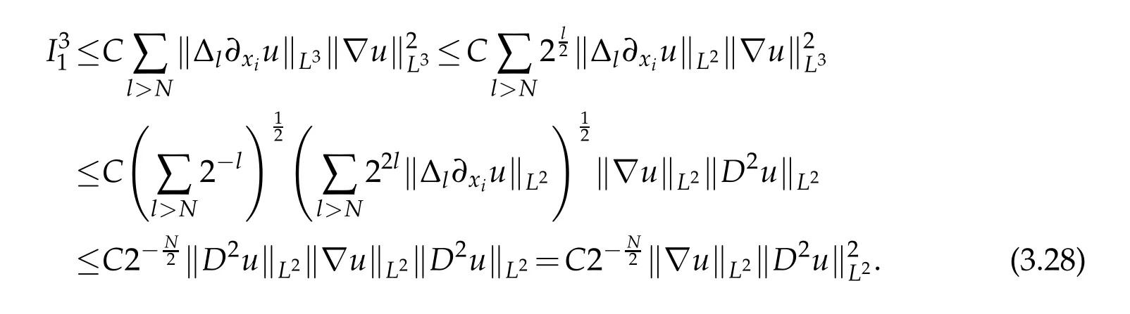
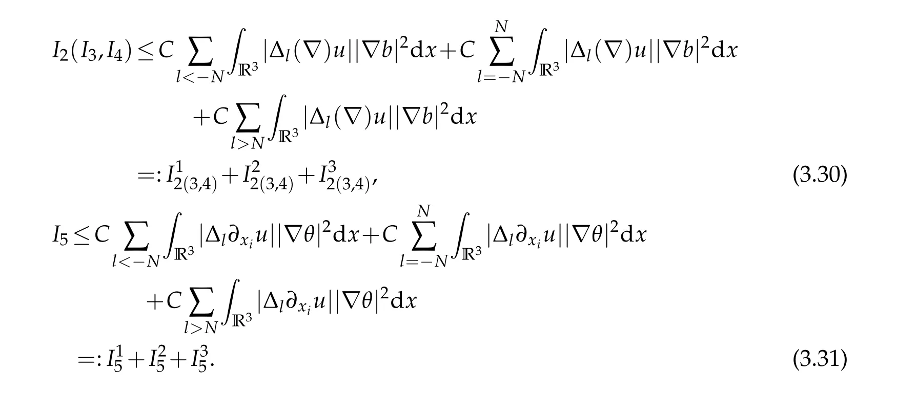
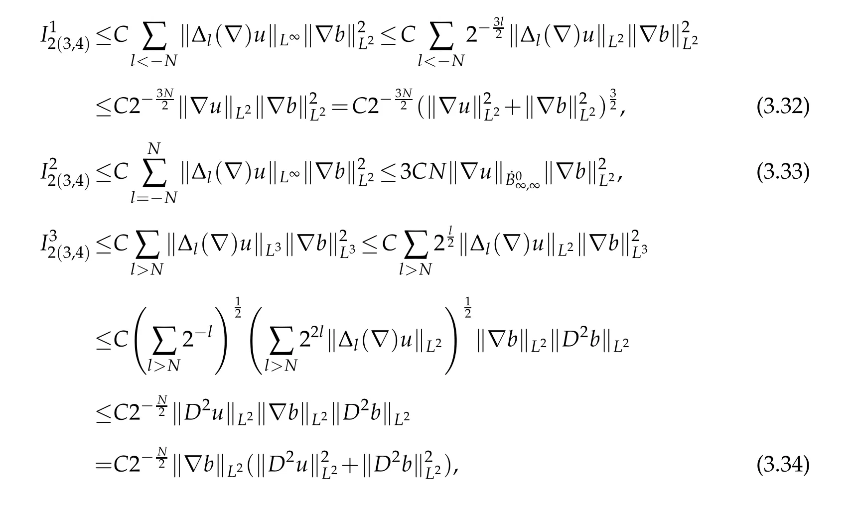
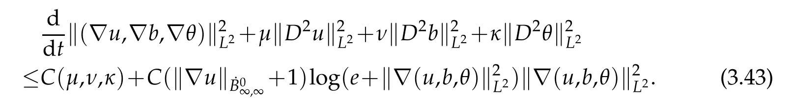
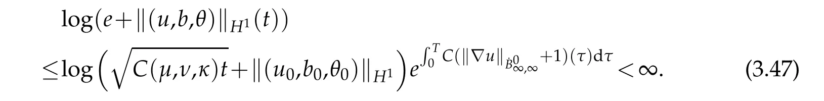
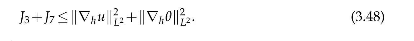
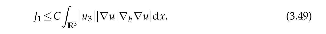
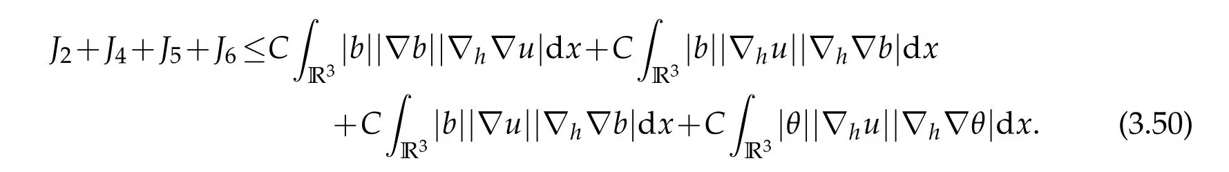
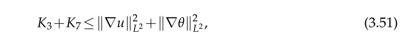
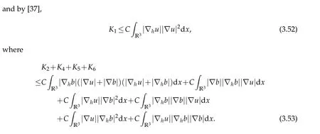
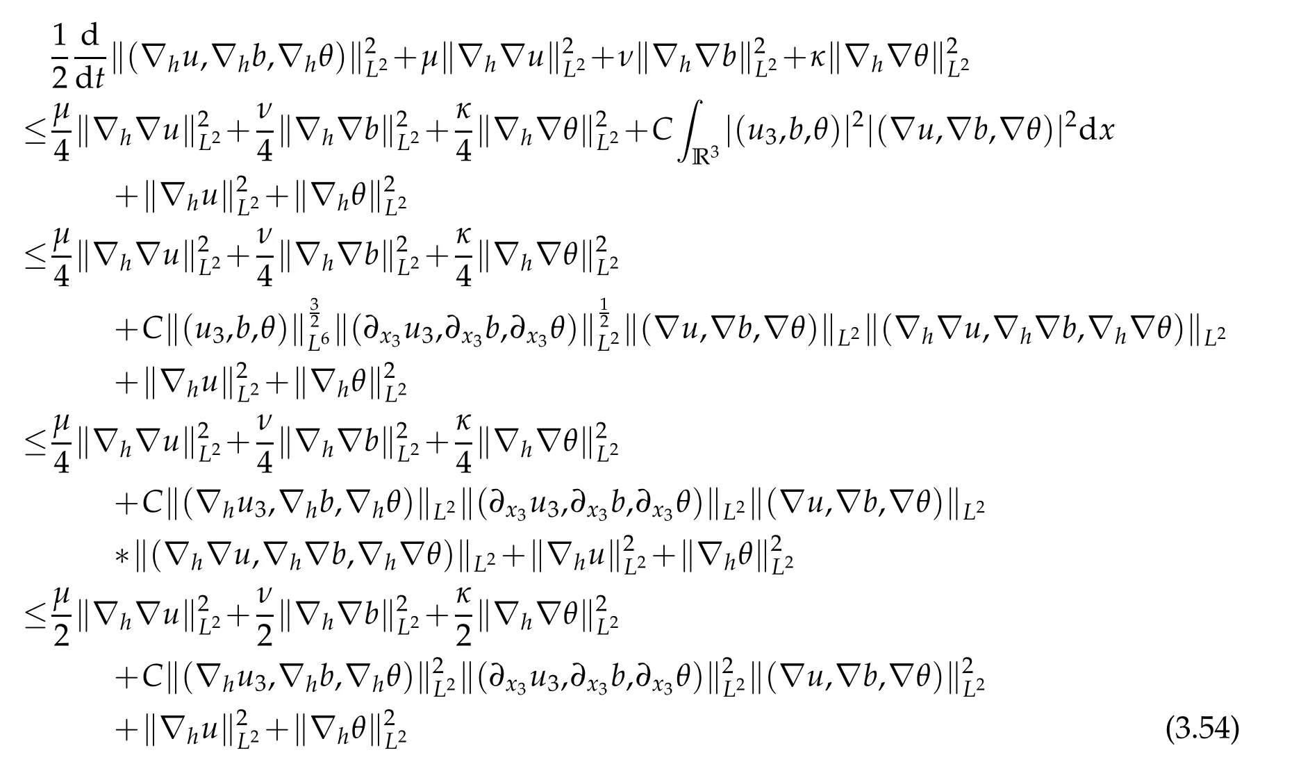
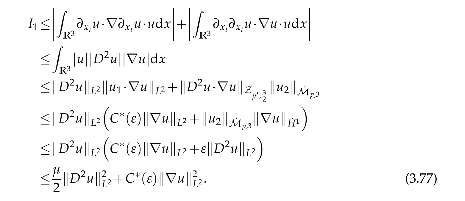
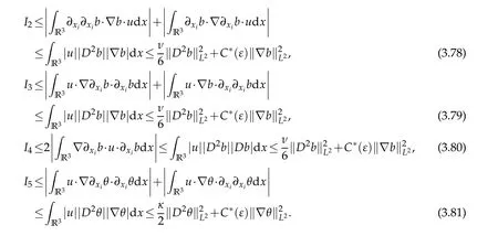
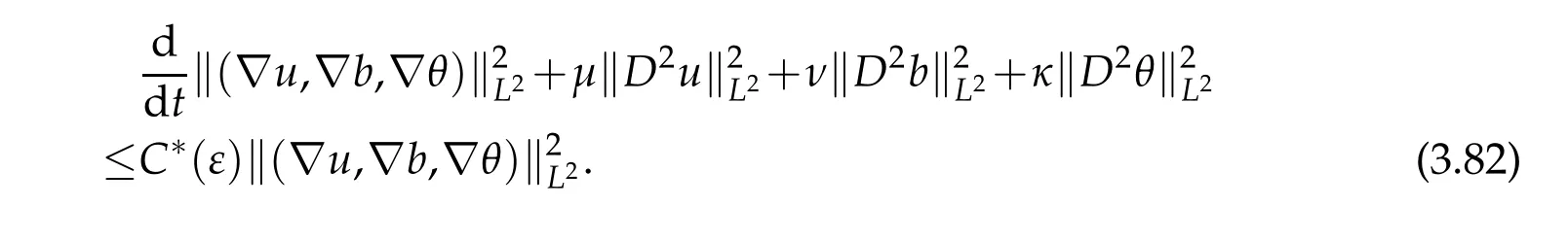
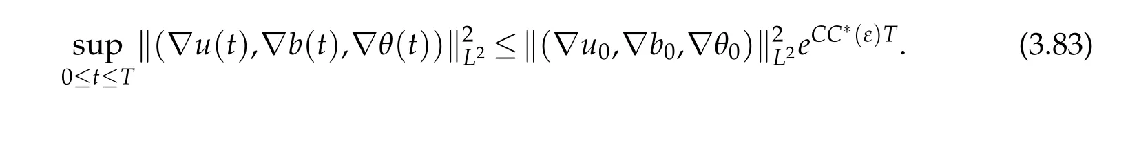
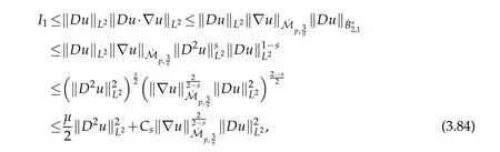
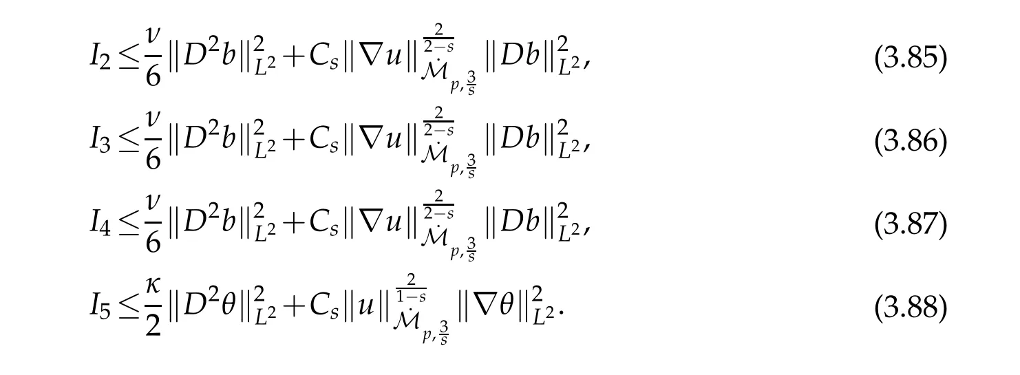
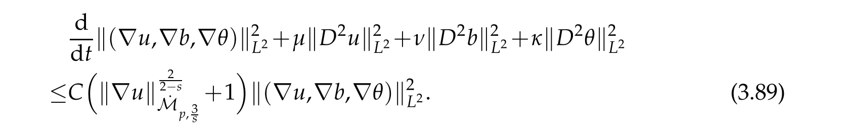
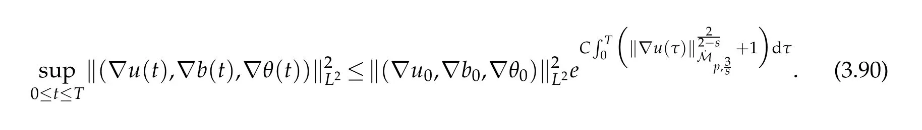
12.Let 1 13.Z′(R3)denotes the dual space of 14.Let 1≤q′≤p′<∞,we define the homogeneous space Zp′,q′as the subspace ofLq′(R3)of functionsf,which can be decomposed into an atomic serieswhere the functionsand satisfy the following inequalities for the diameterdkof the support ofgk:dk≤1 and Zp′,q′is a Banach space when it is equipped with the norm: where the infimum is taken over all possible decompositions offinto an atomic series. 16.Lets∈R,p,q∈[1,∞),the homogeneous Besov spaceis defined by the full-dyadic decomposition such as 17.As usual,constants that appear in this paper may change in value from line to line without change of notation.WithCa,b,cwe denote constants that depend ona,bandc,for example. 18.For conciseness,the short notation has been used in this paper. In this subsection,for readers’convenience,we are first going to recall some basic facts on Littlewood-Paley theory,one may check[29]for more details. Let S(R3)be the Schwartz class of rapidly decreasing functions.Givenf∈S(R3),its Fourier transformis defined by Choose two nonnegative radial functionsχ,ϕ∈S(R3)supported respectively in B=such that SetϕjandandDefine the frequency localization operators: Formally,∆j=Sj+1−Sjis a frequency projection into the annulus{|ξ|≈2j},andSjis a frequency projection into the ball{|ξ|≾2j}.One easily verifies that with the above choice ofϕ By telescoping the series,we thus have the Littlewood-Paley decomposition for allf∈L2(R3),where the summation is in theL2sense. In what follows,we shall make continuous use of Bernstein inequalities,which comes from[29,30]. Lemma 2.1(Chemin[29]and Lemari´e-Rieusset[30]).For all k∈N∪{0},j∈Zand1≤p≤q≤∞,we have,for all f∈S(R3), with c1,c2being positive constants independent of f,j. Taking advantage of Parseval’s equality and Hölder inequality,we can easily obtained the following useful Lemma. Lemma 2.2.Suppose0≤s≤1,then the following inequality holds The following lemma plays an essential role for the proof of our theorems. Lemma 2.3([30]).Forpointwise multiplication is a bounded bilinear operator from L2(R3)×(R3)toZp′,q′(R3),namely,there exists C>0such that for any f∈L2(R3)and Here it is worth particularly mentioning some properties of the space we are going to use.This kind of space plays an important role in studying the regularity of solutions to partial differential equations(see[31,32]and the references therein). It is not hard to verify thatis a Banach space under the norm.Furthermore,it is easy to check the following relation: Hence,for anyf(x,t)defined for both spatial and time variables, for anyλ>0 withfλ(x,t)=λ f(λx,λ2t).Here,the point is that if(u,b,θ)solves the magnetic B´enard fluid system,then so does(uλ,bλ,θλ)for allλ>0.This is so called scaling dimension zero property. Forp≥2,we have the following comparison between the Lorentz spaces and the Morrey-Campanato space: The following lemma gives an equivalence betweenand a multiplier space Lemma 2.4([31]).,the spaceis defined as the space of f(x)such that thenif and only if f∈with equivalence of norms. Throughout the proof of Theorem 1.1 in Section 3,we shall use the following inequalities frequently. Lemma 2.5.For,we have Lemma 2.6([33]).Suppose that f∈L6(R3),∂x3f∈L2(R3),g∈L2(R3)and∇hg∈L2(R3),then it holds that Lemma 2.7([34]).Suppose that f∈H1(R3),∇h f∈Lσ(R3)and ∂x3f∈Lς(R3),then Lemma 2.8([35]).Suppose that f,g,∇hg,k,∂x3k,∇hk∈L2(R3),then In this section,we prove Theorem 1.1 by using the regularity conditions(1.3)-(1.10),respectively.More precisely,we shall show that under one of the conditions(1.3)-(1.10) in Theorem 1.1.Then by standard arguments of continuation of local solutions,we conclude that the solutions(u(x,t),b(x,t),θ(x,t)) can be extended smoothly beyondt=Tprovided that one of the conditions(1.3)-(1.10)holds.In fact,on the one hand,it is necessary to consider ∀ε∈(0,T)such that(∇u,∇b,∇θ)(ρ)∈L2(R3)for anyρ∈(0,ε).It is well-known that for anyε>0 and the maximum time of existenceT,there is a unique strong solutionand obeys=(u,b,θ)(ρ).Thus,(u,b,θ)(t) is regular in R3×(0,T) providedOn the other hand,suppose thatT≤T,in the following,we shall show that‖(∇u,∇b,∇θ)(t)‖L2is uniformly bounded fort∈[ρ,T)or bounded asin Theorem 1.1.However,this boundedness would imply thatcould be extended beyond,which contradicts the definition of.This completes the proof of Theorem 1.1. For clarity,we separate it into several small cases.Before doing,we fist make some preparations. Applyingto both sides of system(1.1),then multiplying both sides by,respectively,integrating over R3,after suitable integration by parts,one obtains where we used the following facts: where〈·,·〉denotes the inner product inL2(R3). Taking operator ∇hto both sides of equations (1.1),then multiplying the resultants with ∇hu,∇hband ∇hθ,respectively,making use of the integration by parts and the incompressibility condition ∇·u=0,we find Applying ∇to both sides of(1.1),testing by ∇u,∇band ∇θ,respectively,then taking the inner products over the space domain R3,we have For brevity of representation,we denote,forT−s≤t Hereswill be chosen a posteriori. •Case 1:Under the condition(1.3) By the Gagliardo-Nirenberg inequality,Hölder inequality and Young inequality,we have In the same way,forI2,I3,I4andI5,it also can be estimated as By the Holder inequality,the last termI6is easily estimated as From the above inequalities and summing overiwith 1≤i≤3,we have Due to the Gronwall inequality,it follows from(3.13)that,for 3 Especially,the above estimates are also valid forp=∞provided we modify them accordingly.More explicitly,we have the following result whenp=∞ Due to the Gronwall inequality,it follows from(3.15)that •Case 2:Under the condition(1.4) For this case,we first estimateI1as follows: Similarly,forI2,we have I3andI4can be treated as the termI2.TermI5can be dealt with in a similar manner.By means of Hölder’s,Gagliardo-Nirenberg’s and Young’s inequalities,we have Now combining the estimates ofIi(1 ≤i≤5) and (3.12),and substituting into (3.1),we are led to The Gronwall inequality implies the a priori estimate The above proof is also valid forp=∞provided we modify it accordingly.In fact,it is sufficient to change(3.20)and(3.21)as follows: The Gronwall inequality implies the a priori estimate •Case 3:Under the condition(1.5) In this case,we use the Littlewood-Paley decomposition to prove the regularity criterion of weak solutions to system(1.1).To derive the regularity condition(1.5)in Theorem 1.1,in contrast,we apply the Littlewood-Paley decomposition to the nonlinear terms,and decompose them into low frequency,middle frequency and high frequency,and estimate each part by different methods as reference in[36]. At the beginning of Section 3,we have derived(3.1)by differentiating equations(1.1)and multiplying with∂xiu,∂xiband∂xiθ,respectively.In what follows,we estimate each termIi(i=1,2,3,4,5) separately.Invoking the Littlewood-Paley decomposition(2.1),we have whereNis a positive integer to be determined.Substituting(3.24)intoI1,we obtain Using Holder’s inequality,Lemma 2.1 and Young’s inequality,I11is dominated as For,from the Hölder inequality and Lemma 2.1,it follows that Finally,can be estimated as In the above calculations,we utilize the Hölder inequality and Lemma 2.1. Summing up estimates(3.26)-(3.28),it follows The other four terms are bounded similarly.For simplicity,we detail the second and fifth one,I2andI5. By virtue of Lemma 2.1 and Hölder’s inequality,we obtain Then Lemma 2.1,Hölder’s inequality,Gagliardo-Nirenberg’s inequality and Young’s inequality imply that Collecting estimates(3.30),(3.32)-(3.34),and(3.31),(3.35)-(3.37),it derives that Now combining the estimates ofIi(i=1,2,3,4,5) and (3.12),and substituting into (3.1),we are led to Now we takeNin(3.40)so that where the constantCmay depend onµ,ν,κ.Then(3.40)implies that Applying Gronwall’s inequality twice,we gather that,for 0≤t The energy inequality(1.2)implies that Thus,we have Taking logarithmic on both sides of (3.46) and applying the Gronwall inequality again,we obtain,for any 0≤t •Case 4:Under the condition(1.6) By using Hölder’s and Young’s inequalities,we have In[37],the authors showed that Moreover,we also have For termsKi,i=1,···,7, Thus,by using Hölder’s and Young’s inequalities and Lemmas 2.6-2.7, and by Lemma 2.8, Thanks to Gronwall’s inequality and together with(1.2)and the regularity condition(1.6),one has •Case 5:Under the condition(1.7) Let us examine termsJi(i=1,2,4,5,6)in an alterative way.More precisely,by[38]and[26], Therefore,by using Lemma 2.8 and Young’s inequality, Besides this,we further have by using Lemma 2.8, which implies it yields that which further infer that Choosing 0 consequently we obtain that for any •Case 6:Under the condition(1.8) By the Hölder inequality and the Young inequality,the first termI1is dominated as where we used the interpolation inequality in Lemma 2.2. Similarly,we can estimateI2as In the same way,forI3,I4andI5,it also can be dominated as From the above inequalities and the estimate (3.12) ofI6,and summing overiwith 1≤i≤3,we have Hence,by using Gronwall’s inequality,we have,for 0 •Case 7:Under the condition(1.9) In the caseu∈C([0,T);,one can decomposeu=u1+u2with for allT>0 and anyε>0.We can choose whereC∗is sufficiently large.We first estimateI1: Similarly,forI2-I5,one has Collecting the above estimates ofI1-I5and the estimate(3.12)ofI6and summing upifrom 1 to 3,it follows that Applying Gronwall’s inequality,we have •Case 8:Under the condition(1.10) For the case 8,we first estimateI1as follows: where we used the interpolation inequality in Lemma 2.2. Similarly,forI2,I3,I4,I5,we have Combining the above estimates and(3.12)and summing overiwith 1≤i≤3,we obtain Due to Gronwall’s inequality,it follows from(3.89)that,for 0 Acknowledgements The author would like to thank professor Lili Du for many helpxful discussions and suggestions.The authors would also like to thank the referee for his/her pertinent comments and advice.The research of L.Ma was supported by the National Natural Science Foundation of China (Nos.11571243,11971331),China Scholarship Council (No.202008515084),Opening Fund of Geomathematics Key Laboratory of Sichuan Province(No.scsxdz2020zd02)and Teacher’s development Scientific Research Staring Foundation of Chengdu University of Technology(No.10912-KYQD2019 07717).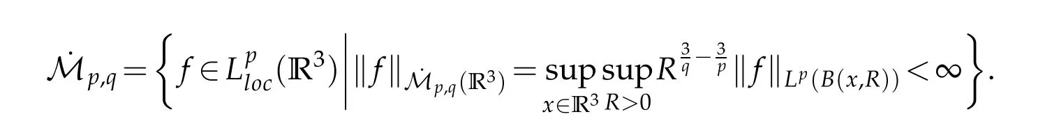


2.2 Auxiliary lemmas


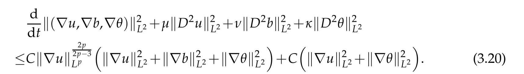
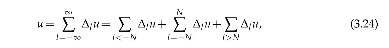
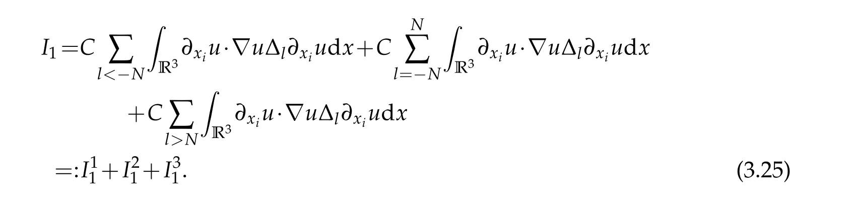
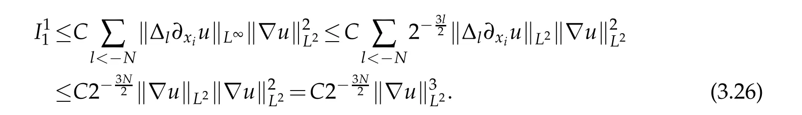
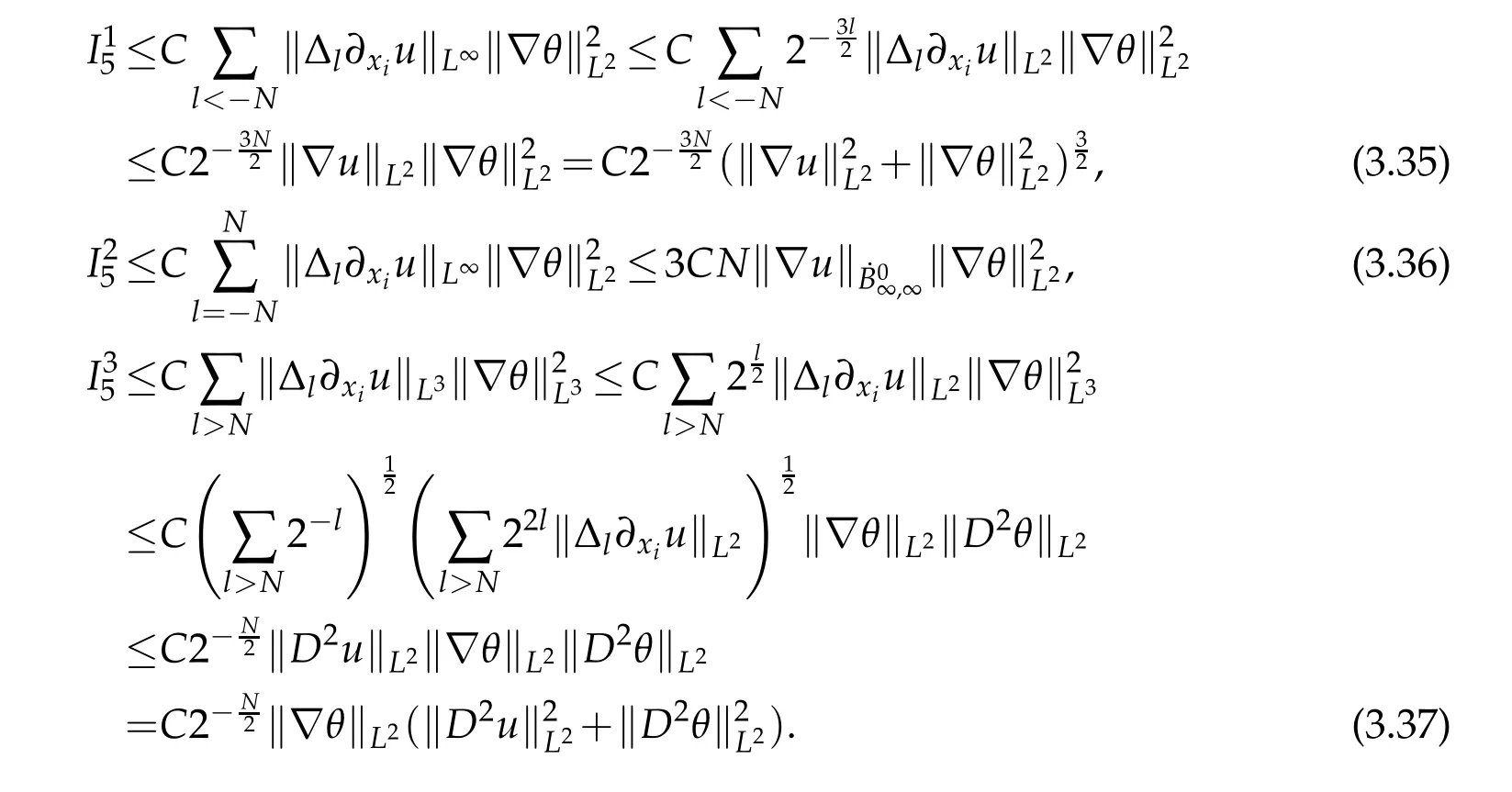
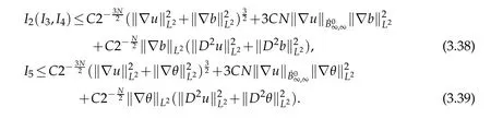
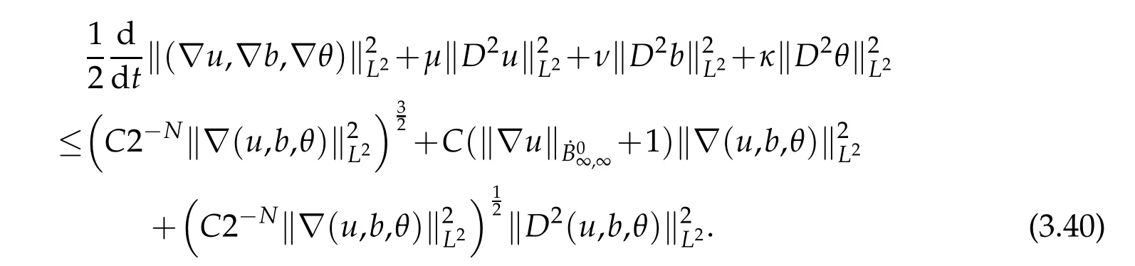
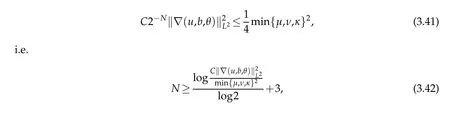
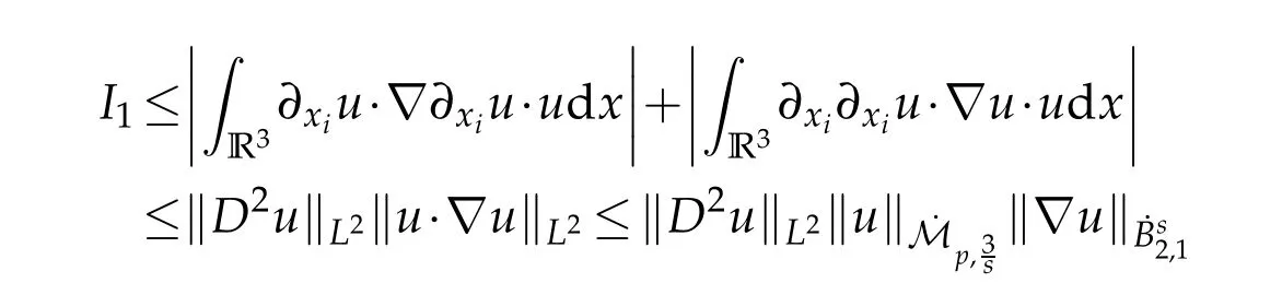
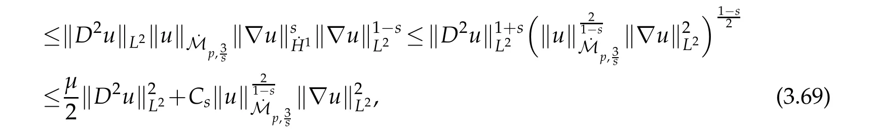
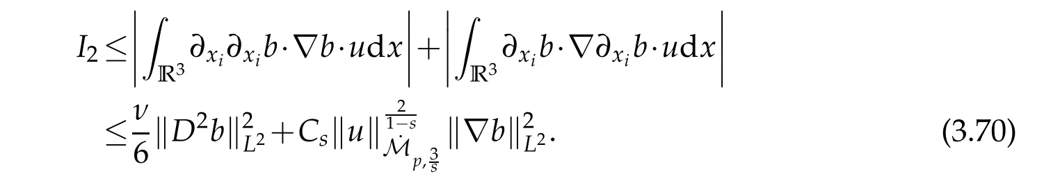
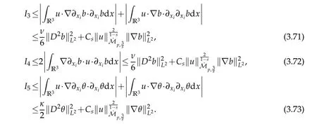
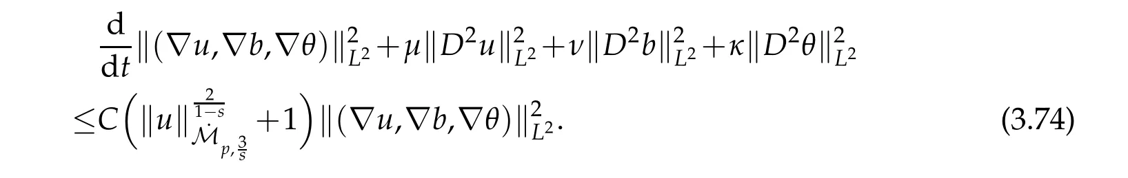
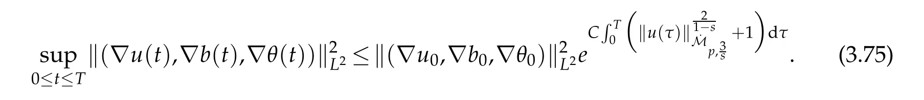
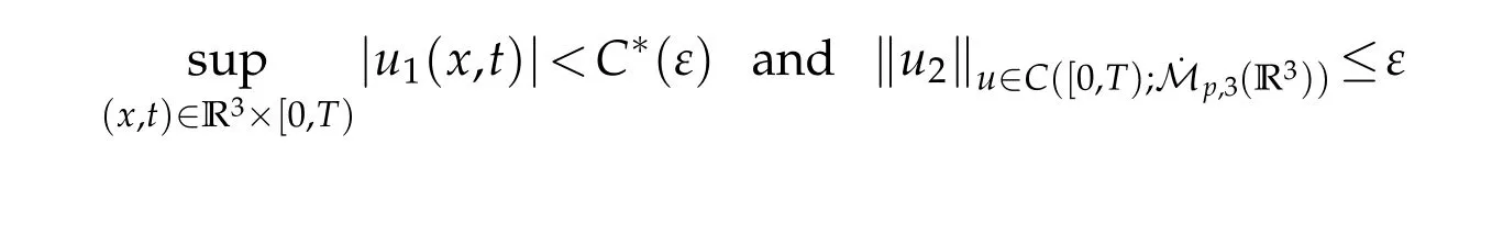
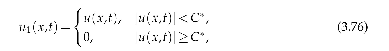
3 Proof of Theorem 1.1


杂志排行

Journal of Partial Differential Equations的其它文章
- Global Attracting Sets of Neutral Stochastic Functional Differential Equations Drivenby Poisson Jumps
- Trudinger-Moser Type Inequality Under Lorentz-Sobolev Norms Constraint
- Asymptotic Behavior in a Quasilinear Fully Parabolic Chemotaxis System with Indirect Signal Production and Logistic Source
- On Existence of Local Solutions for a Hyperbolic System Modelling Chemotaxis with Memory Term
- Existence of Positive Solutions for theNonhomogeneous Schrödinger-Poisson System with Strong Singularity