Wu Lili,Fu Ying

(School of Mathematics,Northwest University,Xi′an 710127,China)

Abstract：In this paper,we are concerned with the persistence properties of solutions of the Cauchy problem associated to an integrable two-component Camassa-Holm system with cubic nonlinearity.It is shown that a strong solution of the two-component Camassa-Holm system,initially decaying exponentially together with its spacial derivative,also decay exponentially at infinity by using weight functions.Furthermore,we give an optimal decaying estimate of the momentum.

Keywords：two-component Camassa-Holm system,persistence properties,optimal decaying estimates

1 Introduction

In this paper,we consider the following initial value problem(IVP)associated with an integrable two-component Camassa-Holm system with cubic nonlinearity

wherem=u−uxx,n=v−vxx.The system in(1)was proposed by Reference[1],so it is also called the SQQ equation.It is proven that the system in(1)is integrable in the sense of not only Lax-pair but also geometry,namely,it describes pseudospherical surfaces.The SQQ equation also possesses infinitely many conservation laws and exact solutions such as cuspons and W/M-shape solitons(see Reference[1]).

The blow-up phenomena of the problem(1)has been developed in several works,for example see References[2-3].The one peaked solitons and two peakon solutions are described in an explicit formula in Reference[2].The Cauchy problem(1)is locally well-posed for initial data(m0,n0)∈Hs(R)×Hs(R)withs≥1 also can be found in Reference[2].

With suitable conditions on the initial data,a global existence result for the strong solution is established in Reference[3].It is also established the local well-posedness for IVP(1)in Besov spaceswith 1≤p,r≤+∞ands>maxin Reference[2].As a special case,Reference[3]investigated the local well-posedness of the IVP(1)in the critical Besov space,and it is shown that the data-to-solution mapping is Hölder continuous.

Apparently,ifu=v,then the system in(1)is reduced to an integrable equation with cubic nonlinearity,which is called the FORQ equation or the modified Camass-Holm equation

In fact,the system in(1)is a generalized version of the equation(2),which was introduced by References[4-6]as a new integrable system by applying the general method of tri-Hamiltonian duality to the bi-Hamiltonian representation of the modified KdV equation.It was shown in Reference[7],the FORQ equation has the bi-Hamiltonian structure and the Lax pair,which implies the integrability of the equation so that the initial value problem may be solved by the inverse scattering transform method.Reference[7]also deveoped a new kind of soliton: “W-shape-peaks”/“M-shape-peaks”solutions by studying the equation(2).It was in Reference[8]shown that the equation(2)allows invariant subspacesW2=L{sinx,cosx}and corresponding exact solution isu(x,t)=λsin|x−λt|,whereλis an arbitrary constant.

A considerable amount of work has been devoted to study the persistence properties of solutions of Cauchy problem,such as the Novikov equation[9],the 2-component Degasperis-Procesi equation[10],the interacting system of the Camassa-Holm and Degasperis-Procesi equations[11],etc.Reference[12]studied the persistence properties and unique continuation of solutions of the Camassa-Holm equation

The main objective of this paper is to study the persistence properties of solutions to the initial value problem(1).In Section 2,we prove the persistence properties of IVP(1)as listed in Theorem 1.1.The proof of the optimal decay index of the momentummandnis in Section 3.

Before stating our main results,let us first present the following well-posedness theorem given in Reference[2].

Lemma 1.1[2]Assume that(m0,n0)∈Hs(R)×Hs(R)withs≥1.There exists a maximal existence timeT=T(‖m0‖Hs(R),‖n0‖Hs(R))>0,and a unique solution(m,n)to the IVP(1)such that

Moreover,the solution depends continuously on the initial data,that is,the mapping:

is continuous.

From the above well-posedness result,we may now utilize it to establish the persistence properties of the solutions to the problem(1).Inspired by Reference[12]for the Camassa-Holm equation,we have the following results.

Theorem 1.1Assume thats≥3,T>0,and

is a solution of the initial value problem(1).If the initial data

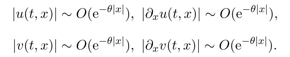
decays at infinity,more precisely,if there exists someθ∈(0,1)such that as|x|→∞,

Then as|x|→∞,we have

Theorem 1.2Givenz0=(u0,v0)∈Hs(R)×Hs(R),s≥3.LetT=T(z0)be the maximal existence time of the solutionsz(t,x)=(u(t,x),v(t,x))to the problem(1)with the initial dataz0.If for someλ≥0 andp≥1,

then for allt∈[0,T),we have

Moreover,if the initial data satisfies

then for allt∈[0,T),we get

Notation 1.1In the following,the convolution is denoted by∗.For a given classical Sobolev spaceHs(R),s>0,we denote its norm by‖·‖Hs.For 1≤p≤∞,the norm in the Lebesgue spaceLp(R)is denoted by‖·‖Lp.Since all spaces of functions are over R,for simplicity,we drop R in our notations of function spaces if there is no ambiguity.We shall say that|f(x)|～O(eax)asx→∞if

2 The proof of Theorem 1.1

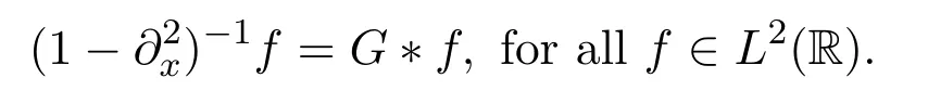
G∗m=u,andG∗n=v.By these identities,it is convenient to rewrite the problem(1)in its formally equivalent integral-differential form

Assume thatz∈C([0,T];Hs)×C([0,T];Hs)is a strong solution of the initial value problem(1)withs≥3.Let

hence by Sobolev imbedding theorem,we have

We now introduce the weight fuction

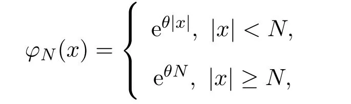
whereN∈N andθ∈(0,1).Observe that for allNwe have

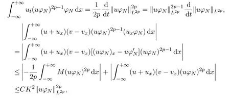
Multiplying the first equation of the problem(7)by(uφN)2p−1φNwithp∈N and integrating the result in thex-variable,we obtain

(8),(9)and Hölder′s inequality lead us to achieve the following estimates

SinceF1,F2∈L1∩L∞andG∈W1,1,we know that∂xG∗F1,G∗F2∈L1∩L∞.Thus,by taking the limit of(11)asp→∞,we get

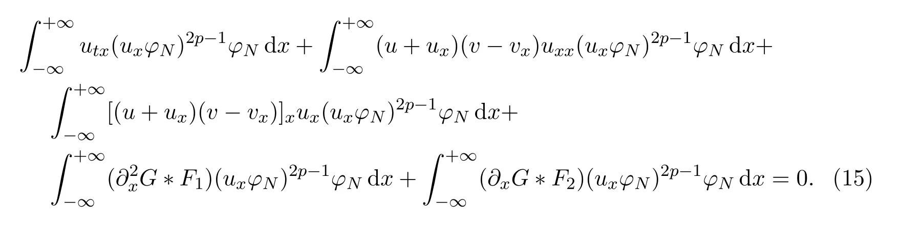
Next,differentiating the first equation of the problem(7)in thex-variable produces the equation

Multiplying(14)by(uxφN)2p−1φNwithp∈N and integrating the result in thexvariable,we obtain

This leads us to obtain the following estimates

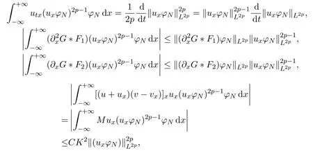
for the second integral of(15),using integration by parts,we estimate as follows

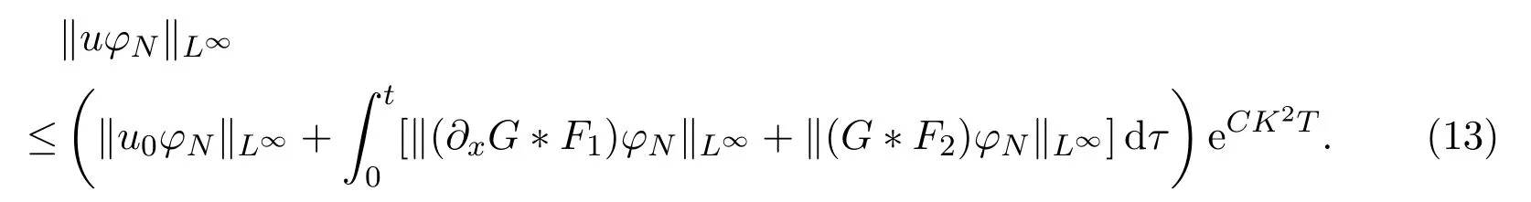
From(15)and the above estimates,we achieve the following differential inequality

by Gronwall′s inequality and lettingp→∞,(16)implies the following estimate

A simple calculation shows that forθ∈(0,1),

Thus,for any functionf,g,h∈L∞,we have

Therefore,sinceu,v,ux,vx,m,n,M∈L∞,we get

whereCis a constant depending onC0,K,andT.

Multiplying the second equation of the problem(7)by(vφN)2p−1φNwithp∈N and integrating the result in thex-variable,then differentiating the second equation of the problem(7)with respect to the spacial variablex,multiplying by(vxφN)2p−1φNand integrating the result in thex-variable,using the similar steps above,we get

Adding(22)and(23)up,we have

Hence,for anyN∈N and anyt∈[0,T],by Gronwall′s inequality we get

which completes the proof of Theorem 1.1.

3 The proof of Theorem 1.2

whereN∈N andλ∈(0,∞).Obviously,for allNwe have

Multiplying the first equation of the problem(1)by(mφN)2p−1φNwithp∈N and integrating the result in thex-variable one gets

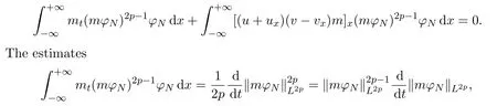
and therefore,by Gronwall′s inequality

As the process of the estimation to(25),we deal with the second equation of the problem(1)

Add up(25)with(26),we have

Thus,by the assumption(3),the inequality(4)holds.

Next,lettingp→∞in(27),we get

In view of assumption(5),we obtain

taking the limit asNgoes to infinity in(28)and combing(28)and(29),we get the result

This completes the proof of Theorem 1.2.