A STABILITY PROBLEM FOR THE 3D MAGNETOHYDRODYNAMIC EQUATIONS NEAR EQUILIBRIUM∗
2021-09-06可雪丽原保全肖亚敏
(可雪丽) (原保全) (肖亚敏)
School of Mathematics and Information Science,Henan Polytechnic University,Henan 454000,China E-mail:kexueli123@126.com;bqyuan@hpu.edu.cn;ymxiao106@163.com
Abstract This paper is concerned with a stability problem on perturbations near a physically important steady state solution of the 3D MHD system.We obtain three major results.The first assesses the existence of global solutions with small initial data.Second,we derive the temporal decay estimate of the solution in the L2-norm,where to prove the result,we need to overcome the difficulty caused by the presence of linear terms from perturbation.Finally,the decay rate in L2space for higher order derivatives of the solution is established.
Key words Background magnetic field;MHD equations with perturbation;stability;decay rate
1 Introduction
The 3D incompressible magnetohydrodynamic equations can be written as
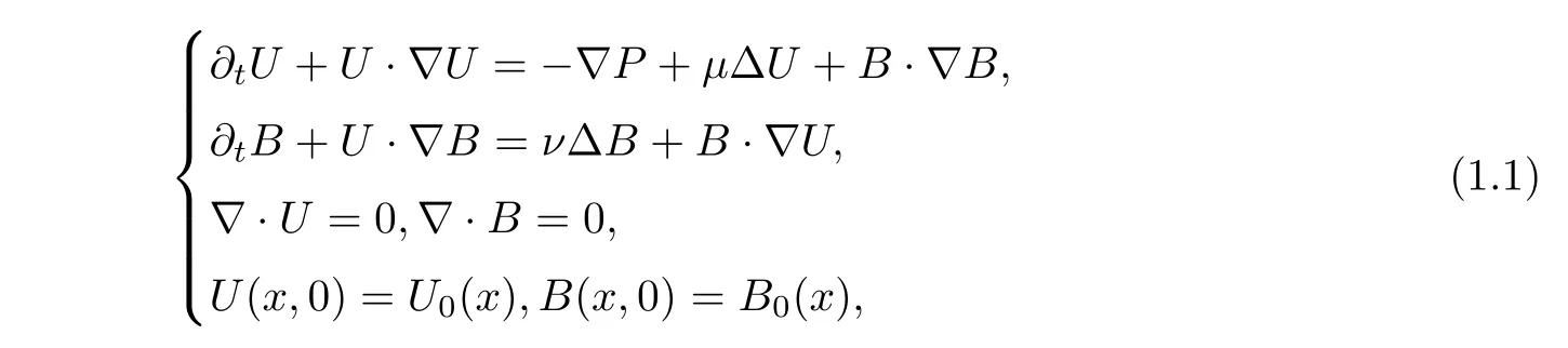
x
∈Randt>
0.U
=U
(x,t
)represents the fluid velocity,B
=B
(x,t
)the magnetic field,andP
=P
(x,t
)the pressure.For simplicity,we set the viscosity coefficientµ
and the magnetic field coefficientν
to 1.The MHD equations(1.1)involve the coupling of the incompressible Navier-Stokes equation and Maxwell’s equation.They play an important role in many fields,such as geophysics,astrophysics,cosmology and engineering(see[3,5,19]).Because of the physical and engineering applications of MHD equations,the mathematical study of them is very important;as a result,the MHD equations have been extensively studied.For instance,G.Duvaut and J.L.Lions[8]obtained the local existence and uniqueness of a solution in the Sobolev spaceH
(R),s>d,
and proved the global existence of the solution for small initial data.M.Sermange and R.Teman[25]further studied the properties of the solutions.Miao,Yuan and Zhang[18]studied the well-posedness of solutions of MHD equations in BMO(R)andbmo
(R),and proved that the solution of the Cauchy problem of MHD with small initial value is globally unique in BMO(R)and locally unique inbmo
(R).Cao,Wu and Yuan[4]studied the 2D incompressible MHD with partial dissipation for data inH
(R),s>
2.Recently,the global regularity issue concerning equations(1.1)has attracted much interest,and considerable results have been obtained(see[9,11,29]).For the 3D equations around the equilibrium state(U
,B
),it is clear thatU
(x,t
)=(0,
0,
0)andB
=(1,
0,
0)are the special solutions of(1.1).The perturbation(u,b
)around this equilibrium withu
≜U
−U
,b
≜B
−B
obeys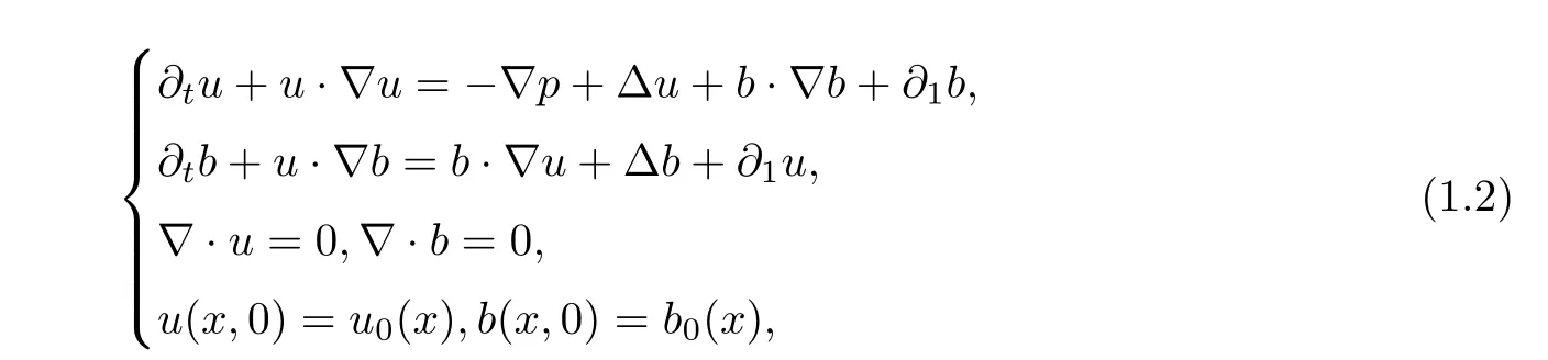
x
∈R,t>
0.
H
(R).For the global solution of equations(1.2),we refer to[16,27].For the decay estimation of equations(1.2),we refer to[7,15,21,24].However,the classical method does not apply here,due to the appearance of linear terms∂
u
and∂
b
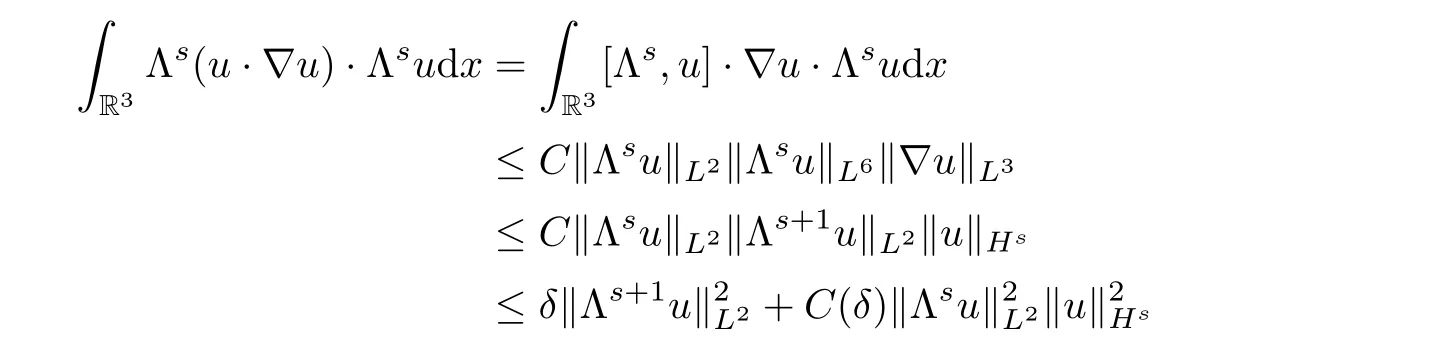
from the perturbation in equations(1.2).We introduce a diagonalization method to eliminate the linear terms,then we prove the temporal decay estimates by the classical Fourier splitting method.Our main results are stated as follows:First,to prove the global well-posedness of small initial data in Theorem 1.2,we need the local well-posedness result of the strong solution in Proposition 1.1,which can be obtained by a standard procedure with Friedrichs’method.The key estimate is that
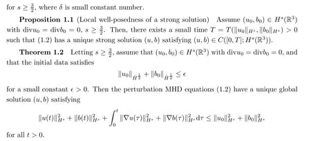


The decay rate of the higher order derivative of the solution is also obtained.
Theorem 1.4
Under the assumption of Theorem 1.3,for any integerm
≥0,the small global solution(u,b
)satis fies
C
is a constant which depends onm
and the initial data.Λ=√−∆is de fined in the end of this section.Remark 1.5
The decay rates(1.3)and(1.4)are optimal in the sense that they coincide with the ones of the heat equation.Remark 1.6
For the real numbers>
0,we can also obtain the time decay rate of theL
−norm for thes
-order derivative of the solution by the interpolation relation
m<s<m
+1,which is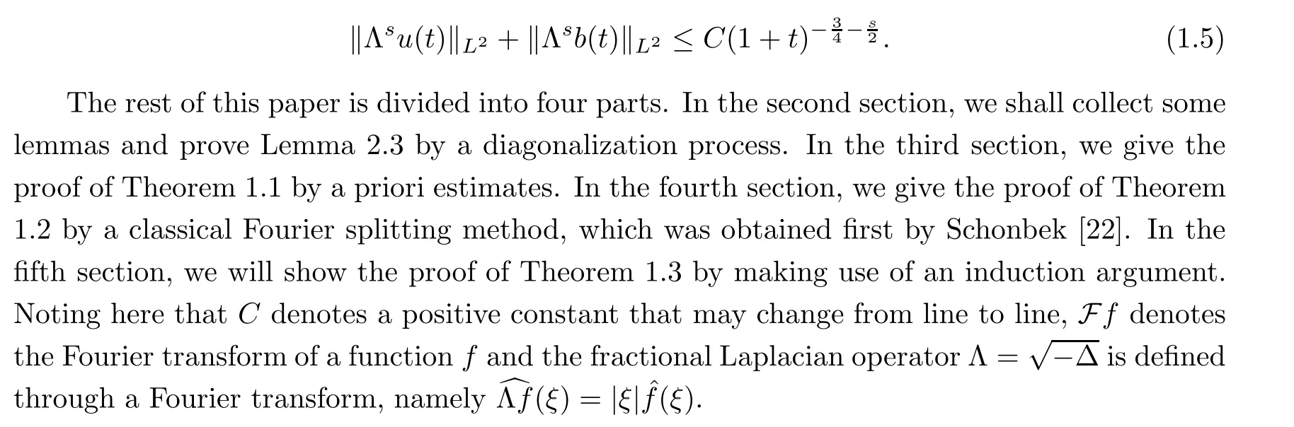
2 Preliminaries
The primary purpose of this section is to give three Lemmas;the first one is the product type estimate,the second and the third are mainly used for the decay estimate of a solution.The detailed processes are as follows:
Lemma 2.1
(Product estimate[13,14,17])Let 1<p<
∞,ands>
0.Then there exists a constantC
such that
L
estimate of the Fourier transform of the initial datum in a ball(the proof of Lemma 2.2 is based on the Hausdorff-Young theorem;for more details please refer to[12,22,30]):Lemma 2.2
Letu
∈L
(R),1≤p<
2.Then
S
(t
)={ξ
∈R:|ξ
|≤g
(t
)}is a ball with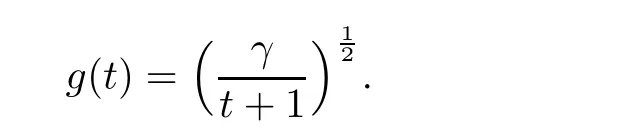
γ>
0 is a constant which will be determined later,and C is a constant which depends uponγ
and theL
norm ofu
.In order to prove Theorem 1.2,we need to calculate the estimates of|u
︿(ξ
)|and|︿b
(ξ
)|,which will play a key role in this paper.For more details,readers can refer to[7,26].Lemma 2.3
Letting(u,b
)∈C
([0,T
];H
(R))be a global solution to the Cauchy problem(1.2)with initial data(u
,b
)∈L
(R)∩H
(R),there exists a constantC>
0 depending only on‖u
‖and‖b
‖such that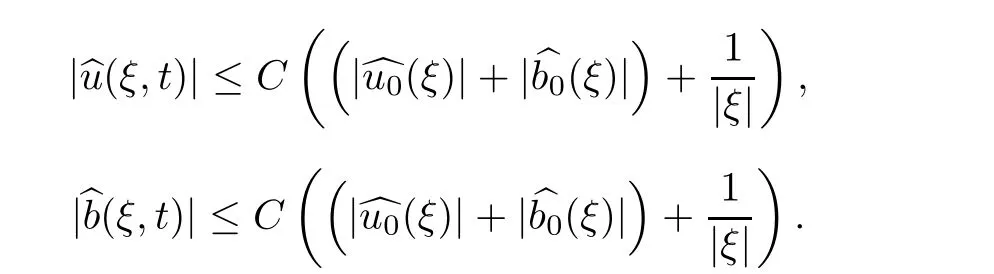
Proof
We rewrite(1.2)in the following form:
G
:=−u
·∇u
+b
·∇b
−∇p
,F
:=−u
·∇b
+b
·∇u.
We take the Fourier transform for(2.3)as

Then the eigenvalues of matrix A can be calculated as follows:

The associated eigenvectors are
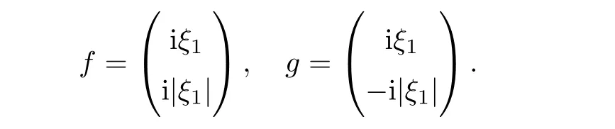
C
of the eigenvectors and its inverse are given by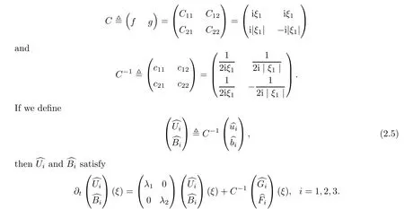
Integrating in time,by Duhamel’s formula,we have

i
=1,
2,
3,and,according to(2.5),we have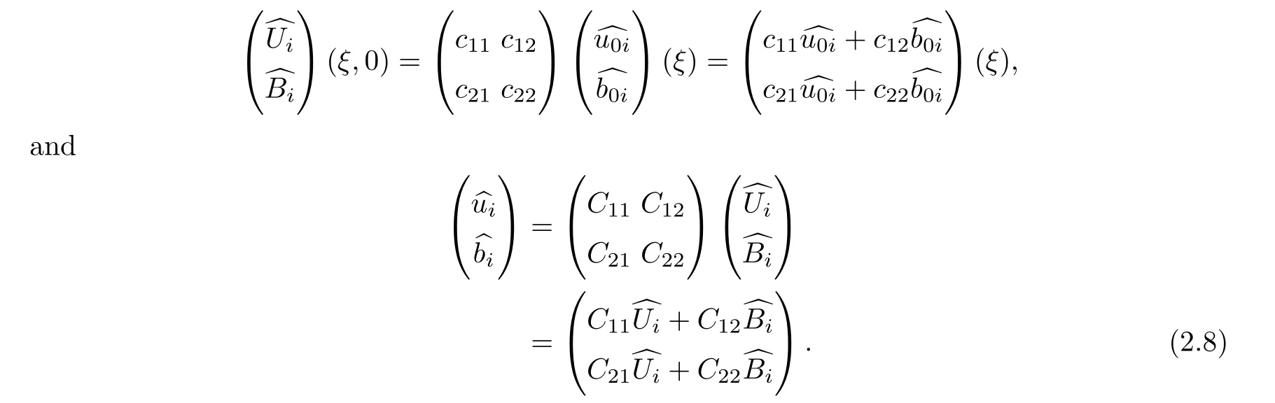
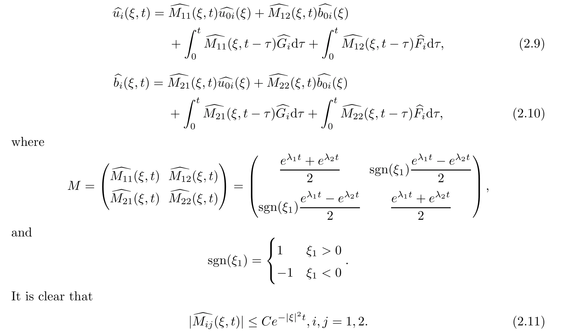
We can get from(2.6)–(2.8)that
u
andb
,we have
L
toL
,this leads to
u
andb
,we can obtain that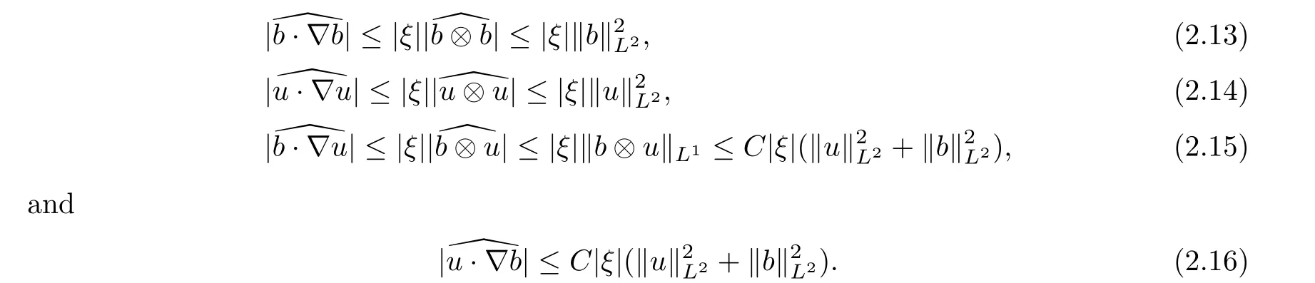
G
andF
,we get
Inserting(2.17),(2.18)and(2.11)into(2.9),we deduce that


Using an argument similar to(2.10),we have

The proof of Lemma 2.3 is thus completed.
3 Proof of Theorem 1.2

3.1 L2estimate
Taking theL
inner products of the equations(1.
2)withu
andb
,and adding the results and integrating by parts,we obtain
where we have used the fact that

3.2 Hsestimate
Applying Λto the equations of(1.2),dotting the resulting equations with Λu
and Λb
,and integrating over R,we have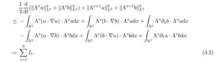
I
–I
.For the termI
,by the divergence free condition ofu
,integration by parts,Lemma 2.1 and‖f
‖≤C
‖f
‖,we obtain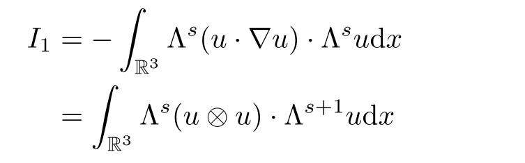
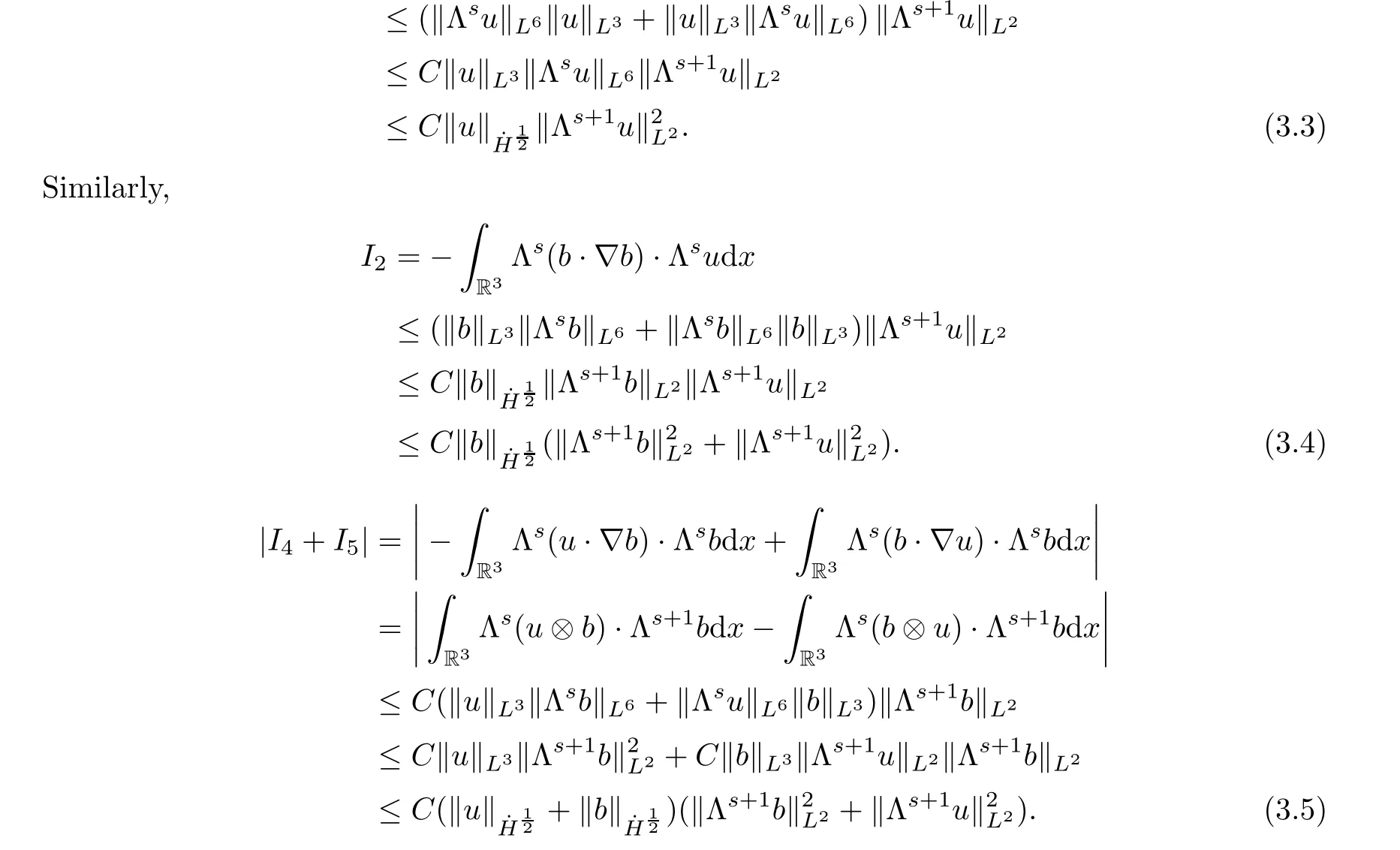
I
andI
,integrating by parts,we get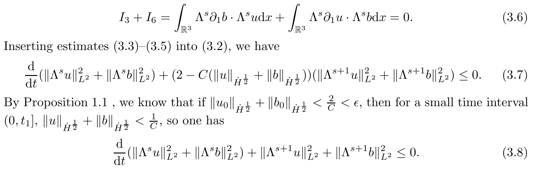
Combining this with estimate(3.1),we have
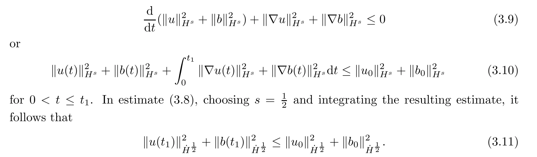
Thus,by a continuous extending argument,we get

<t<
∞.This completes the proof of Theorem 1.1.4 Proof of Theorem 1.3
In this section,we prove the decay rate of the global solution inL
(R)by the classic Fourier splitting method.Proof
Applying Plancherel’s theorem to(3.1),and by splitting the phase space Rinto two time-dependent parts,we get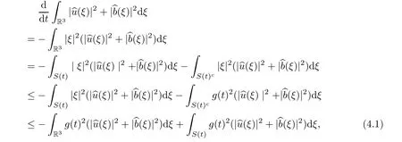
S
(t
)andg
(t
)are de fined in Lemma 2.2,andγ>
0 is a constant which will be determined later.Thus,we obtain
t
+1),it follows that
By Lemma 2.3,we have

t
leads to the result


S
(t
),
Similarly,we obtain

Inserting(4.7)and(4.8)into(4.3),and by Lemma 2.2,we have



This completes the proof of Theorem 1.2.
5 Proof of Theorem 1.4
In this section,we will prove the higher order derivative’s decay estimate of the small global solution to the equations of(1.2)inL
(R)space.Proof
We use the Fourier splitting method again.Let
Then Plancherel’s theorem and(5.1)imply that
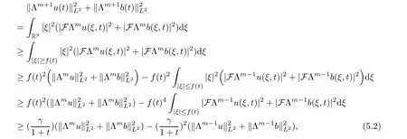
m
≥1 is an integer.Inserting estimate(5.2)into(3.8),it follows that
m
=1,multiplying both sides of inequality(5.3)by the integrating factor(t
+1)yields
t
,we have


m>
1,
Therefore,inserting the above estimate into(5.3),we have

t
),we obtain
,t
],we get
Therefore,the proof of Theorem 1.3 is completed.
杂志排行

Acta Mathematica Scientia(English Series)的其它文章
- REGULARITY OF WEAK SOLUTIONS TO A CLASS OF NONLINEAR PROBLEM∗
- EXISTENCE TO FRACTIONAL CRITICAL EQUATION WITH HARDY-LITTLEWOOD-SOBOLEV NONLINEARITIES∗
- A DIFFUSIVE SVEIR EPIDEMIC MODEL WITH TIME DELAY AND GENERAL INCIDENCE∗
- ON A COUPLED INTEGRO-DIFFERENTIAL SYSTEM INVOLVING MIXED FRACTIONAL DERIVATIVES AND INTEGRALS OF DIFFERENT ORDERS∗
- CLASSIFICATION OF SOLUTIONS TO HIGHER FRACTIONAL ORDER SYSTEMS∗
- ENERGY CONSERVATION FOR SOLUTIONS OF INCOMPRESSIBLE VISCOELASTIC FLUIDS∗