(何一鸣)

School of Mathematics and Statistics,Central China Normal University,Wuhan 430079,China E-mail:18855310582@163.com

Ruizhao ZI (訾瑞昭)†

School of Mathematics and Statistics&Hubei Key Laboratory of Mathematical Sciences,Central China Normal University,Wuhan 430079,China E-mail:rzz@mail.ccnu.edu.cn

Key words Incompressible viscoelastic fluids;weak solutions;energy conservation

1 Introduction

In this paper,we consider the issue of energy conservation for solutions to the incompressible viscoelastic flows

where u∈Rdenotes the velocity of the fluid,F is the deformation tensor in a set of

d

×

d

matrices with detF=1(that is the incompressible condition),

FF

=

τ

,which is the Cauchy-Green strain tensor,

P

is the pressure of the fluid,and

µ

≥0 is the coefficient of viscosity.For a given velocity field u(

x,t

)∈R,one de fines the flow map

x

(

t,X

)by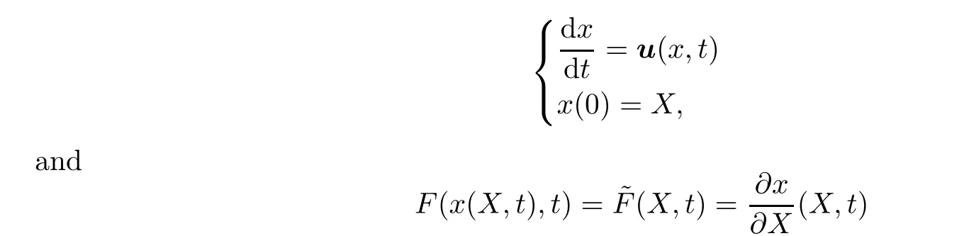

is the Jacobian of the flow map

x

(

t,X

).Moreover,the initial data satisfy

For when the coefficient of the viscosity is

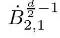
µ

=0,the global existence in 3D whole space was established by Sideris and Thomases in[37,38]by using the generalized energy method of Klainerman[24].The 2D case is more delicate,and here the first non-trivial long time existence result was obtained by Lei,Sideris and Zhou[27]by combining the generalized energy method of Klainerman and Alinhac’s ghost weight method[2].Lei[26]proved the 2D global well-posedness of the classical solution by exploring the strong null condition of the system in the Lagrangian coordinates.Wang[39]gave a new proof in Euler coordinates.In this paper,we are interested in the energy conservation of weak solutions to incompressible viscoelastic fluids(1.1).More precisely,our question is how badly behaved(u

,

F)can keep the energy conservation

and

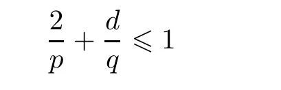
d

is the dimension of space.In[35],Shinbrot showed that Serrin’s condition can be replaced by a condition independent of dimension,that is,u∈

L

(0

,T

;

L

(Ω)),where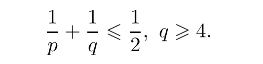

Recently,Yu,in[40],gave a new proof of Shinbrot’s result.

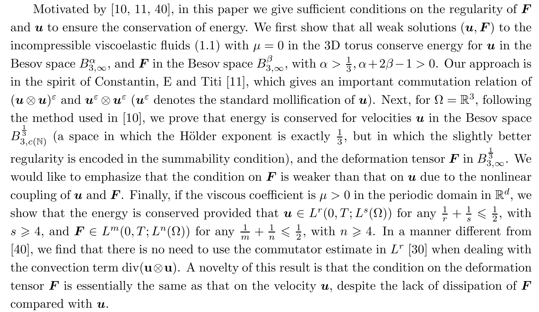
Before proceeding any further,we would like to give some notations which will be used throughout the paper.

Notations

(1)Throughout the paper,

C

stands for a positive harmless“constant”.The notation

f

≾

g

means that

f

≤

Cg

.(2)Let(divM)=

∂

M

,where

M

is a

d

×

d

matrix;(∇u)=

∂

u

;Fis the transpose of the matrix F=(F

,

···

,

F),where Fis the

j

-th column of F.

De finition 1.1

We say that(u

,

F)is a weak solution of(1.1)with Cauchy data(1.2),if it satis fies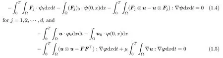

for any test vectors ϕ

,

ψ∈

C

([0

,T

)×Ω;R)with compact support,and divϕ=0.

Our main results are stated as follows:

Remark 1.3

Compared with the general result in[21],our result in Theorem 1.2 allows

u

and

F

to possess different regularities.

Our second result is built on R.

Finally,we investigate the case of

µ>

0 in the torus T.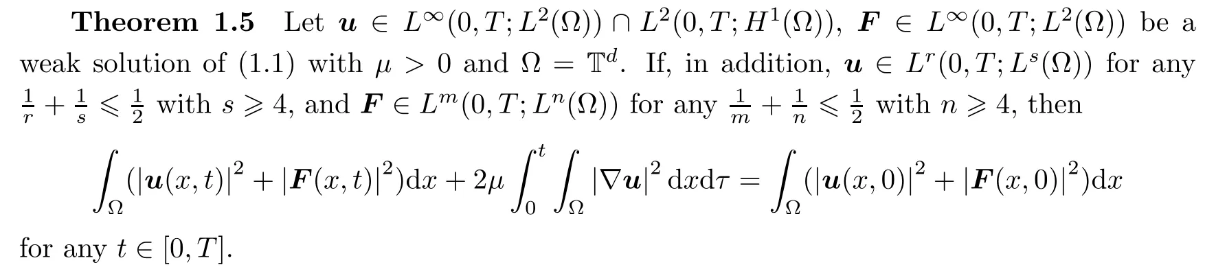

Remark 1.6

It would be very interesting to investigate the boundary effect,and we will consider this problem in the near future.

2 Preliminaries

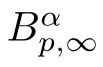
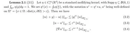
Corollary 2.2

For two functions

u,v

,let us denote

where

δ

u

(

x

)=

u

(

x

−

y

)−

u

(

x

).Then the identity

Remark 2.3

(2.5)is a general case of(10)in[11].

Then,the following is true:

For Q∈N,the low frequency cut-offoperator

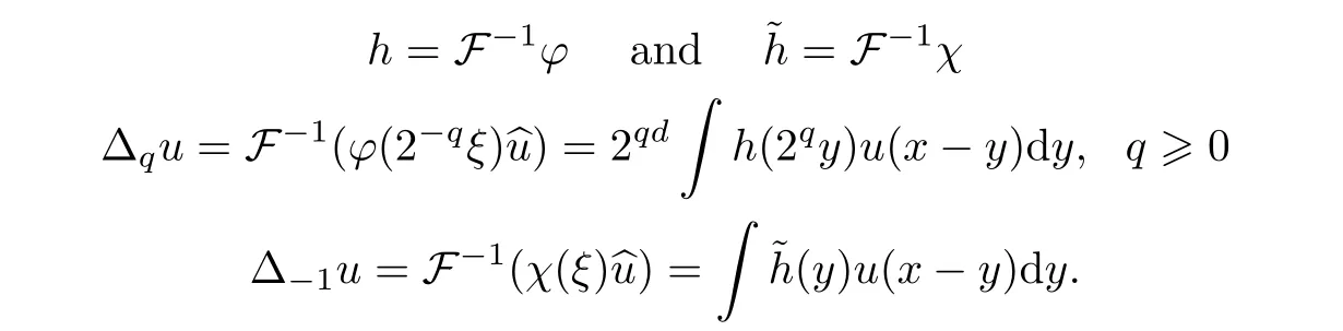
S

u

is de fined by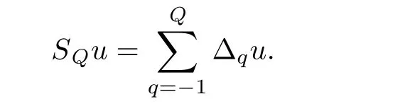

We then have

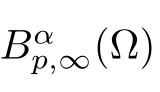
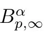
With the aid of the Little wood-Paley decomposition,Besov spaces can also be de fined as follows:

is finite.

The following lemma describes the way derivatives act on spectrally localized functions:

Lemma 2.6

(Bernstein’s inequalities[3])Letting C be an annulus and B a ball,a constant

C

exists such that for any nonnegative integer

k

,any couple(

p,q

)∈[1

,

∞]with

q

≥

p

≥1,and any function

u

of

L

,we have

In particular,we have

As a consequence,we have the following inclusions:

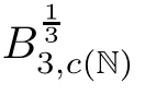
The following space was first introduced by Cheskidov et al.in[10]:

Finally,we would like to introduce a crucial lemma for commutator estimates in

L

.For a proof of this lemma,please refer to[30].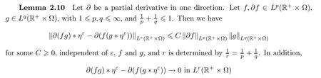

3 Proof of the Results

3.1 Proof of Theorem 1.2

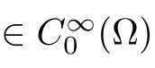
We will use the summation convention for notational convenience.For the sake of simplicity,we will proceed as if the solution is differentiable in time.The extra arguments needed to mollify in time are straightforward.

Now,using(u)and(F)to test the first and second equations of(1.1),one obtains

which in turn gives

Integrating by parts,using(2.5)in Corollary 2.2,and noting that div

u

=0,we have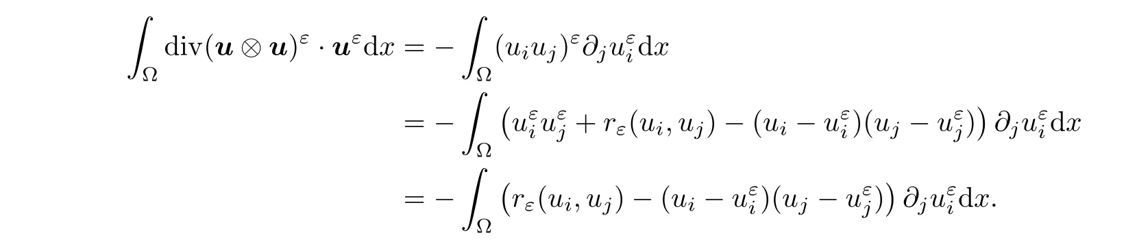

Similarly,we have

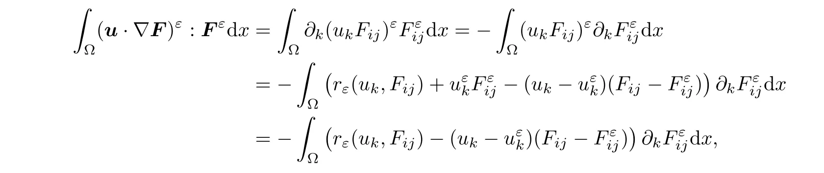
due to the fact that

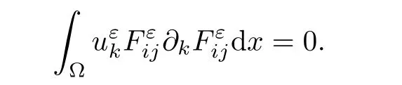
In the same way,we have

Finally,noting that divF=0,

Thanks to the fact that divF=0,integrating by parts,we are led to

Now,adding the two equations in(3.1)together,using the equalities obtained above,and recalling that

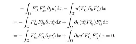
µ

=0,we get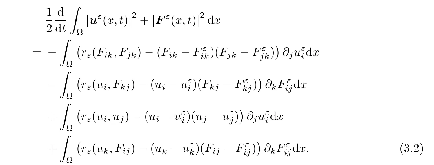

Then,integrating(3.2)w.r.t.the time variable,one deduces that

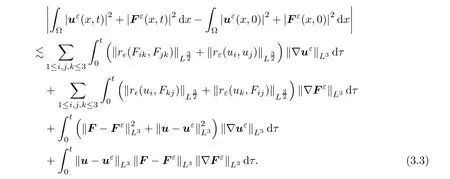
By Corollary 2.2,we have

Combining this with Lemma 2.1,it follows that if 3

α

−1

>

0

,α

+2

β

−1

>

0,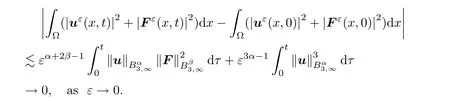

We complete the proof of Theorem 1.2.

3.2 Proof of Theorem 1.4

Let us start this subsection by introducing the following localization kernel as in[10]:

For tempered distribution

u

and

F

in R,denote

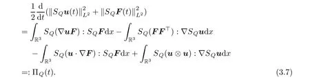
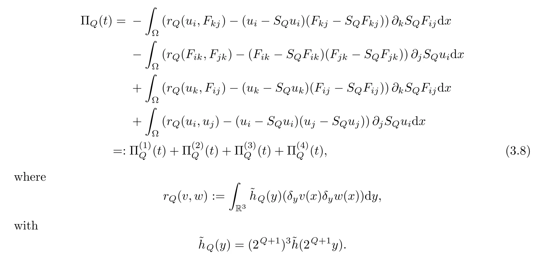
In a fashion similar to(3.2),after cancelation,we arrive at

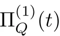
By Minkowski’s inequality,

Let us now use Bernstein’s inequalities and Remark 2.8 to estimate

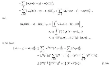
Similarly,it holds that

On the other hand,

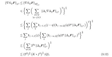
and similarly,

Noting that(3.10)and(3.11)also imply

respectively,it then follows from(3.9)–(3.14)that

In the same manner,we have

Accordingly,

From this estimate and Young’s inequality,noting that‖

K

‖

<

∞,we immediately obtain

3.3 Proof of Theorem 1.5

We shall complete the proof of Theorem 1.5 by the following two steps:

In fact,(3.22)is obviously true if

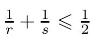
r

≥4,so we only consider the case in which 2≤

r<

4 and

s>

4.By interpolation,

for some

θ

∈(0

,

1).It suffices to show that there exists a

θ

∈(0

,

1)such that

To this end,we choose

θ

satisfying

This makes sense,because for 2≤

r<

4 and

s>

4,

We will use(3.22)and(3.24)frequently in the next proof.

Step(II)

By(3.1),it is easy to verify that

Integrating in time and adding the two equations together,we have

We next rewrite

due to the fact that divF=0.Moreover,

Substituting the above four equalities into(3.25),thanks to divu=0,we find that

as

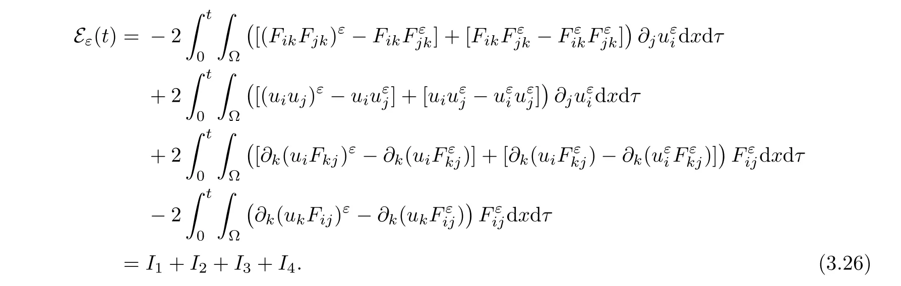
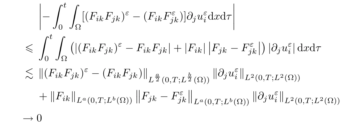
ε

tends to zero,and that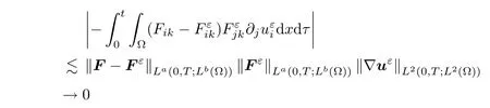

as

ε

→0.It follows that

In the same way,we obtain

For the term

I

,Lemma 2.10 ensures that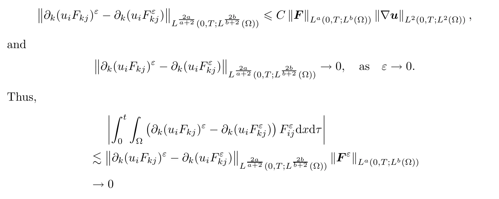

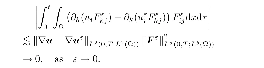
It follows that

Finally,in view of Lemma 2.10,

as

ε

→0.Letting

ε

go to zero in(3.25),and using(3.27)–(3.30),we obtain

This completes the proof of Theorem 1.5.