Zihao Zong,Tielin Shi and Qi Xia

The State Key Laboratory of Digital Manufacturing Equipment and Technology,Huazhong University of Science and Technology,Wuhan,China

ABSTRACT A parameter-free approach is proposed to determine the Lagrange multiplier for the constraint of material volume in the level set method.It is inspired by the procedure of determining the threshold of sensitivity number in the BESO method.It first computes the difference between the volume of current design and the upper bound of volume.Then,the Lagrange multiplier is regarded as the threshold of sensitivity number to remove the redundant material.Numerical examples proved that this approach is effective to constrain the volume.More importantly,there is no parameter in the proposed approach,which makes it convenient to use.In addition,the convergence is stable,and there is no big oscillation.

KEYWORDS Lagrange multiplier;threshold of sensitivity;BESO method;level set method;topology optimization

1 Introduction

Among many methods for structure topology optimization[1–14],the level set method[5–10]has caught much attention.Determining the Lagrange multiplier for the constraint of material volume is an indispensable task in the level set method[15].A straightforward approach to complete this task is to gauss a Lagrange multiplier and keep it fixed during the optimization[8],but this simple approach cannot accurately enforce the volume constraint.The second approach relies on averaging certain quantity on the boundary being optimized[9],for instance the Lagrange multiplier for the minimal compliance problem is obtained as the average of the density of strain energy on the boundary.Although this approach can accurately enforce the volume constraint,the integration on a boundary is cumbersome.The third approach is to adjust the Lagrange multiplier according to the volume of material,and it is called the augmented Lagrange multiplier method[16–18].This approach can also accurately enforce the volume constraint.However,it is often difficult to guess a proper value of the penalty parameter in this method,hence considerable oscillations of compliance and volume usually happen as the optimization progresses.In fact,the penalty parameter significantly affects the optimization,and an improper value of the penalty parameter may even make the optimization not converge.

The approaches reviewed above are successful to determine the Lagrange multiplier.In our present study,a new approach is proposed,i.e.,a parameter-free approach using the bi-directional evolutionary structural optimization(BESO)method[12,19–21].It is inspired by the procedure for determining a threshold for material deletion and addition in the BESO.Currently,there is a trend of combining different methods of structural topology optimization[22–29]to give full play to their advantages and to complement each other,hence leading to a more powerful topology optimization method.In[22–24,28],the BESO was respectively integrated into the level set method and the phase field method to nucleate holes.In[26,27]the density method was integrated into the level set method.In[25,29]the level set method was used in the BESO to obtain smooth boundary of structures.Through the combination of different methods of structural topology optimization,several drawbacks were successfully overcome.The present study offers still another combination between the BESO method and the level set method.

2 The Level Set Based Topology Optimization

The boundaryΓobeing optimized of a structureΩis described by the zero isocontour of the signed distance functionΦ(x)ofΓo.Let structures stay within a fixed domainD,i.e.,Ω⊂D.Then,we have

Propagation ofΓois described by the Hamilton-Jacobi(H–J)equation

whereθnis the velocity ofΓoin its outward normal direction.

The compliance minimization problem given by Eq.(2)is considered here minC(u)

whereCis the objective function;a(u,v)=ℓ(v)is the weak form equation;Vis the volume of material;is the upper bound.The design velocity for the optimization problem Eq.(2)is given by

whereAe(u)·e(u)is the density of strain energy;λis the Lagrange multiplier for the constraint of material volume.Whenθn>0 the structure expands and the volume increases.Whenθn<0 the structure shrinks and the volume decreases.Finally,whenθn=0 the structure does not change and the optimization converges.

Now,an important task is to determineλin Eq.(3).There are several approaches to complete this task[15].A straightforward approach is to gauss a Lagrange multiplier and keep it fixed during the optimization[8],but this simple approach cannot accurately enforce the volume constraint.The second approach is the boundary integration approach[9]where the Lagrange multiplier is obtained as the average strain energy density according to Eq.(3),i.e.,

Although this approach can accurately enforce the volume constraint,the integration along boundaryΓois cumbersome.The third approach is the augmented Lagrange multiplier[18,24].In this approach,λis adjusted according to the volume of material,i.e.,

whereτ >0 is a penalty parameter;kdenotes the current iteration of optimization.Again,this approach can accurately enforce the volume constraint.However,it is often difficult to guess a proper value of the penalty parameterτin this method,hence considerable oscillations of compliance and volume usually happen during the optimization.In fact,the penalty parameterτsignificantly affects the optimization,and an improper value ofτmay even make the optimization not converge.

When the volume of current design is larger than,the structure is required to shrink to satisfy the volume constraint,and according to Eq.(3)this calls for a larger value of the Lagrange multiplier.Similarly,when the volume of current design is smaller than,the volume constraint is not active,and the structure is allowed to expand to reduce its compliance.More importantly,when the optimization converges,we haveV=andθn=0 according to Eq.(3),and the accurate valueλ∗of the Lagrange multiplier is equal to the uniform strain energy density on the optimized boundary,i.e.,

Such an observation offers us the theoretical background to determine the Lagrange multiplier for the constraint of material volume in the level set method by using the BESO method.

3 Determining λ for the Level Set Method by Using the BESO

3.1 The BESO Method

BESO[12,19–21]uses sensitivity number to achieve deletion and addition of material.In the present study,the sensitivity number of thee-th element is given by[12,19]

where k0is the stiffness matrix of element;Veis the volume of element.One can see that the first term in right hand side of Eq.(3)and the sensitivity number Eq.(7)are both the strain energy density.According to the BESO method[12,19],a spatial filtering is first applied to the sensitivity numbers,i.e.,Then,a temporal smoothing is applied,i.e.,.

3.2 Determining λ for the Level Set Method

Inspired by the process in the BESO method for determining the thresholdαth for design updating,a new approach is proposed to determineλin the level set method.

In every optimization iteration,we first compute the difference between the volume of current design(denoted asVk)andin Eq.(2),i.e.,

IfΔVk≤0,we setλ=0.IfΔVk >0,the procedure of determining the thresholdαth is adapted to determine the Lagrange multiplier,and it is described as follows:

In order to delete the redundant materialΔVk,suppose thatNΔsolid elements need to be removed from the current design.First,for all the solid elements,we sort their sensitivity numbers so thatThen,the Lagrange multiplier is determined as

In other words,the Lagrange multiplier is regarded as the threshold of sensitivity number to remove the redundant material.

Recall that the sensitivity numberin Eq.(9)is smoothed by spatial filtering.Therefore,the strain energy density in Eq.(3)is also smoothed by spatial filtering,and the result is taken as the naturally extended velocity to solve the H-J equation.Otherwise,the Lagrange multiplier given by Eq.(9)may result in an error in volume of the optimized structure.

As one can see in Eqs.(8)and(9),there is no parameter in the procedure to determine the Lagrange multiplier.Such a parameter-free approach is convenient to use,which is important to solve practical engineering problems.On the contrary,the widely used augmented Lagrange multiplier method is often criticized about the penalty parameter that greatly affect the results of optimization.

Note that besides using the BESO method to determine the Lagrange multiplier,we can also use it to nucleate holes during the level set based topology optimization.The details of the hole nucleation are referred to our previous papers[22–24].Nevertheless,the method proposed in the present paper only deals with the Lagrange multiplier and has nothing to do with the hole nucleation.

4 Numerical Examples

In the following examples,the properties of solid material are:E=1 andν=0.3;and those of artificial weak material are:E=1×10−3andν=0.3.We assume the plane stress state and use 4-node bilinear square element.The move limit strategy[30]is applied.In each iteration of optimization,Γois evolved 10 steps and reinitialization is applied toΦ(x).

The criteria of convergence include[19]:

and

In addition,we will terminate the optimization whenk=200.

4.1 Example 1

Fig.1 shows the design optimization problem,and.In the finite element analysis 160×80 elements are used;in the level set computations a grid with 161×81 nodes is used.

Figure 1:Design problem of Example 1

First,we do the optimization with the Lagrange multiplier being determined by using the BESO.Fig.2 shows the initial structure and the optimized structure,and Fig.3 shows the history of optimization.As can be seen in Fig.3,small oscillations of compliance and volume ratio appear after the 100-th iteration.Such small oscillations have no big influence on the results of optimization.In our view,the reason of these oscillations is that the volume ratio of the structure has a small error as compared with the value required by the optimization problem.

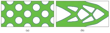
Figure 2:The initial structure and optimized structure with the Lagrange multiplier being determined by using the BESO.Compliance of(b)is 60.50,and volume is 1.00(a)Initial structure(b)Optimized structure

Figure 3:History of the optimization with the Lagrange multiplier being determined by using the BESO

Second,the optimization is done with the Lagrange multiplier being determined by using the augmented Lagrange multiplier method.Fig.2a shows the initial structure.The penalty parameter in Eq.(5)is set toτ=10−3,andλis updated after the 30-th iteration according to the augmented Lagrange multiplier method.In this example,the strain energy density given by the finite element analysis is directly taken(not smoothed by spatial filtering)to compute the naturally extended velocity.Fig.4 shows the optimized design,and Fig.5 shows the history of optimization.From Figs.4 and 2b,we find out that the two optimized structures are similar to each other.Such results prove that the proposed parameter-free approach to determine the Lagrange multiplier is effective.

Figure 4:The optimized structure with the Lagrange multiplier being determined by using the augmented Lagrange multiplier method.Compliance of the optimized structure is 61.53,and volume is 1.00

As can be seen in Fig.5,afterλis updated(i.e.,after the 30-th iteration),obvious oscillations of compliance and volume ratio appear,which is a typical behavior of this method.Such oscillations may significantly change the shape or topology of the structure,and it adversely affects the performance of structure,i.e.,the compliance in the present study.

Figure 5:History of the optimization with the Lagrange multiplier being determined by using the augmented Lagrange multiplier method

From Figs.3 and 5,we can see that there are two different kind of oscillations.First,when the optimization is near to the convergence,as can be seen in Fig.3,the oscillations are very small,and they have no big influence on the results of optimization.Second,as shown in Fig.5,whenλis updated after the 30-th iteration according to the augmented Lagrange multiplier method,significant oscillations arise.Such big oscillations are usually very harmful to the results of optimization,and they should be avoided.

4.2 Example 2

The design optimization problem is shown in Fig.6,andV= 3.Since the structure is symmetric,the right half is considered in the optimization.In the finite element analysis 150×50 elements are used;in the level set computations a grid with 151×51 nodes is used.

Figure 6:Design problem of Example 2

First,the optimization is done with the Lagrange multiplier being determined by using the BESO.Fig.7 shows the initial structure and the optimized structure,and Fig.8 shows the history of optimization.As can be seen in Fig.8,small oscillations of compliance and volume ratio appear after the 70-th iteration.Such small oscillations have no big influence on the results of optimization.

Figure 7:The initial structure and optimized structure with the Lagrange multiplier being determined by using the BESO.Compliance of the optimized structure is 183.19,and volume is 3.00(a)Initial structure(b)Optimized structure

Figure 8:History of the optimization with the Lagrange multiplier being determined by using the BESO

Second,the optimization is done with the Lagrange multiplier being determined by using the augmented Lagrange multiplier method.Fig.7a shows the initial design.The penalty parameter in Eq.(5)is set toτ=10−3,andλis updated after the 30-th iteration according to the augmented Lagrange multiplier method.The strain energy density is directly taken(i.e.,not smoothed by spatial filtering)to compute the velocity to solve the H-J equation.Fig.9 shows the optimized design,and Fig.10 shows the history of optimization.Again,we can see that obvious oscillations appear afterλis updated(i.e.,after the 30-th iteration).

Figure 9:The optimized structure with the Lagrange multiplier being determined by using the augmented Lagrange multiplier method.Compliance of the optimized structure is 187.36,and volume is 3.00

Figure 10:History of convergence of the optimization with the Lagrange multiplier being determined by using the augmented Lagrange multiplier method

Third,we put more holes into the initial design;we use a mesh with 600×200 elements for the finite element analysis and a grid with 601×201 nodes for the level set computation.Then,the optimization is done with the Lagrange multiplier being determined by using the BESO.Fig.11 shows the initial structure and the optimized structure,and Fig.12 shows the history of optimization.With more holes in the initial structure,the shape and topology of the optimized structure appear to be different.

Figure 11:The initial structure and optimized structure with the Lagrange multiplier being determined by using the BESO.Compliance of the optimized structure is 183.01,and volume ratio is 0.50(a)Initial structure(b)Optimized structure

Because the finite element mesh is finer,the threshold of sensitivity number becomes more accurate,and the Lagrange multiplier obtained by Eq.(9)is more accurate.Therefore,as can be seen in Fig.12,there is no oscillation of compliance and volume ratio during the optimization.

Figure 12:History of the optimization with the Lagrange multiplier being determined by using the BESO

4.3 Example 3

The design optimization problem is shown in Fig.13,andV= 3.Since the structure is symmetric,only the right half is considered in the optimization.In the finite element analysis 600×200 elements are used;in the level set computations a grid with 601×201 nodes is used.

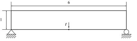
Figure 13:Design problem of Example 3

First,we do the optimization with the Lagrange multiplier being determined by using the BESO.Fig.14 shows the initial structure and the optimized structure,and Fig.15 shows the history of optimization.As can be seen in Fig.15,small oscillations of compliance and volume ratio appear after the 120-th iteration.Fig.16 shows serval intermediate designs,and one can see that the optimization first defines the solid outer skin of the structure,meanwhile many small holes are remained in the inner region.At this time,the porous inner region may be regarded as a region filled with microstructures.Then,as the optimization progresses,some thin beams appear in the optimized structure.

Figure 14:The initial structure and optimized structure with the Lagrange multiplier being determined by using the BESO.Compliance of the optimized structure is 182.93,and volume is 3.00(a)Initial structure(b)Optimized structure

Figure 15:History of the optimization with the Lagrange multiplier being determined by using the BESO

Figure 16:Intermediate designs of the third example with the Lagrange multiplier determined by using BESO(a)Step 20(b)Step 5(c)Step 60(d)Step 80

Second,besides using the BESO to determine the Lagrange multiplier,we also use the BESO to nucleate hole.The details of the hole nucleation are referred to our previous papers[22–24].Fig.17 shows the initial structure and the optimized structure,and Fig.18 shows the history of optimization.One can see that the converge is smooth.Several intermediate designs are shown in Fig.19.

Figure 17:The initial structure and optimized structure with the Lagrange multiplier and hole nucleation achieved by using BESO.Compliance of the optimized structure is 183.79,and volume ratio is 0.50(a)Initial structure(b)Optimized structure

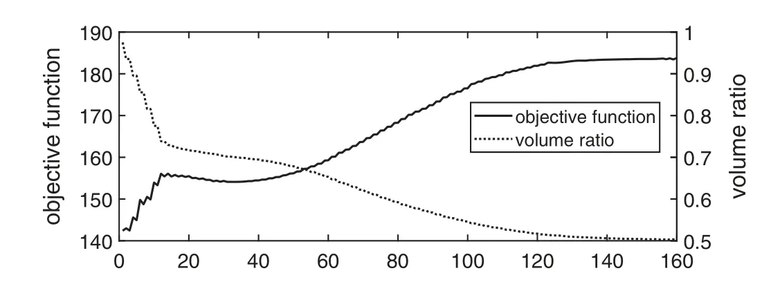
Figure 18:History of convergence of the optimization with the Lagrange multiplier and hole nucleation achieved by using BESO

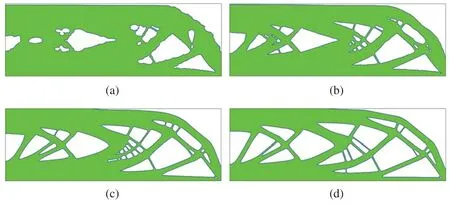
Figure 19:Intermediate designs of the third example with the Lagrange multiplier and hole nucleation achieved by using BESO(a)Step 10(b)Step 20(c)Step 70(d)Step 110

5 Conclusion

Determining the Lagrange multiplier for the constraint of material volume is an indispensable task in the level set method.Although the approaches that can be found in the literature are successful,they also suffer from some drawbacks.In this paper,a new approach is proposed to determine the Lagrange multiplier.First,it computes the difference between the volume of current design and the upper bound of volume.Then,the Lagrange multiplier is regarded as the threshold of sensitivity number to remove the redundant material.Several numerical examples demonstrated that this approach is effective.More importantly,there is no parameter in the proposed approach,which makes it convenient to use.In addition,the convergence is stable,and there is no big oscillation.In the future,the proposed approach will be further extended to deal with other optimization problems or other constraints,for instance,the microstructure optimization[31]or the fatigue damage[32].

Funding Statement:This research work is supported by the National Natural Science Foundation of China(Grant No.51975227).

Conflicts of Interest:The authors declare that they have no conflicts of interest to report regarding the present study.