Haojie Lian,Zhongwang Wang,Haowen Hu,Shengze Li,Xuan Peng and Leilei Chen2,

1Key Laboratory of In-Situ Property-Improving Mining of Ministry of Education,Taiyuan University of Technology,Taiyuan,030024,China

2School of Architecture and Civil Engineering,Huanghuai University,Zhumadian,463003,China

3College of Architecture and Civil Engineering,Xinyang Normal University,Xinyang,464000,China

4Artificial Intelligence Research Center,National Innovation Institute of Defense Technology,Beijing,100071,China

5Department of Mechanical Engineering,Suzhou University of Science and Technology,Suzhou,215009,China

ABSTRACT This paper presents a novel framework for stochastic analysis of linear elastic fracture problems.Monte Carlo simulation(MCs)is adopted to addressthe multi-dimensional uncertainties,whose computation cost is reduced by combination of Proper Orthogonal Decomposition(POD)and the Radial Basis Function(RBF).In order to avoid re-meshing and retain the geometric exactness,isogeometric boundary element method(IGABEM)is employed for simulation,in which the Non-Uniform Rational B-splines(NURBS)are employed for representing the crack surfaces and discretizing dual boundary integral equations.The stress intensity factors(SIFs)are extracted by M integral method.The numerical examples simulate several cracked structures with various uncertain parameters such as load effects,materials,geometric dimensions,and the results are verified by comparison with the analytical solutions.

KEYWORDS Monte Carlo simulation;POD;RBF;isogeometric boundary element method;fracture

1 Introduction

Uncertainties are ubiquitous in engineering applications that may arise from different sources such as inherent material randomness,geometric dimensions,manufacturing errors,and dynamic loading.Because deterministic analysis fails to characterize randomness field,stochastic analysis techniques have been extensively studied to strengthen the credibility of computational prediction of uncertainty problems[1].There are three main variants of stochastic analysis:perturbation based techniques[2],stochastic spectral approaches[3,4],and Monte Carlo simulation(MCs)[5–7].Among them,the MCs is regarded as the most versatile and simplest approach,and often used as the reference solution to verify the results of Perturbation method and Spectral method,but the exhaustive sampling in MCs leads to a heavy computational burden arising from both solving physical problems and constructing analysis-suitable geometric models that must be addressed carefully.

Combining Proper Orthogonal Decomposition(POD)and Radial Basis Functions(RBF)[8–11]is an effective technique of model order reduction[12–14].The POD represents the solution field with the special ordered orthogonal functions in a low-dimensional subspace,which is constructed based on a discrete number of system responses obtained from the evaluation of the full order models(FOM)[15].POD reduces the degrees of freedom by capturing the dominant components of high-dimensional processes because it offers the optimal basis in the sense that the approximation error is minimal inL2norm.On the other hand,the RBF builds a surrogate model through interpolating the data in the reduced space,whereby it admits continuous approximation of system responses for any arbitrary combination of input parameters[16]and thus does not need to solve partial differential equation for each sample.

The pre-processing time of MCs in constructing geometric models can be reduced with isogeometric analysis(IGA)[17].The key idea of IGA is employing spline functions used to construct geometric models in Computer Aided Design(CAD),for example Non-Uniform Rational B-splines(NURBS),T-splines[18],PHT-splines[19,20],and subdivision surfaces[21],as the basis functions to discretize physical fields.Compared to traditional Lagrange polynomial based methods,the main advantage of IGA lies in its ability of integrating numerical analysis and CAD.IGA enables one to perform numerical analysis directly from CAD models without meshing,which is particularly beneficial to uncertainty qualification since it requires fast generation of a large number of models.IGA also offers the benefits of geometric exactness,flexible refinement scheme and high order continuity that are amenable to numerical analysis.

Fracture mechanics is crucial in structural integrity assessment and damage tolerance analyses,but simulation of fracture behaviors poses significant challenges to Finite Element Methods(FEM)for the following reasons:(1)the mesh in proximity to cracks should be several orders of magnitude finer than that used for stress analysis;(2)a remeshing procedure is inevitable when cracks extend;(3)stress singularity or high stress gradients need to be captured.The extended finite element method(XFEM)incorporates enrichment functions to solution space and thus allows for crack propagation in a fixed mesh,but it still relies on a fine and good-quality mesh and necessitates special techniques to represent crack surfaces like Level Set Method.In comparison,Boundary Element Method(BEM)[22–26]has proven a useful tool for fracture simulation.Since BEM only discretizes the boundary of the domain,it not only reduces the degrees of freedom and facilities mesh generation,but more importantly,extends the crack by simply adding new elements at the front of cracks.In addition,as a semi-analytical method,BEM evaluates stress more accurately which is critical in extracting stress intensity factors.Furthermore,isogeometric analysis within the context of boundary element method(IGABEM)inherits the advantage of IGA in integration of CAD and numerical analysis and that of BEM in dimension reduction.IGA with BEM is also natural because both of them are boundary-represented.Since its inception,IGABEM has been successfully applied to potential[27–31],linear elasticity[32–36],acoustics[37–44],electromagnetics[45],structural optimization[40,46–49],etc.,Peng et al.[50,51]applied IGABEM to two dimensional and three dimensional linear elasticity fracture mechanics,and demonstrates the accuracy and efficiency of IGABEM in this area.

This paper presents a novel procedure for solving uncertainty problems of fracture mechanics.In this method,the IGABEM is employed for fracture analysis,and MCs for addressing multiple random parameters.The computational cost is reduced by combination of POD and RBF.The remaining of this paper is structured as follows.Section 2 introduces the fundamentals of MCs in stochastic analysis.Section 3 illustrates how to apply POD and RBF to MCs.Section 4 formulates IGABEM in linear elasticity fracture mechanics.Several numerical examples are given in Section 5 to test the reliability,accuracy and efficiency of the proposed method,followed by conclusions in Section 6.

2 Stochastic Analysis with Monte Carlo Simulation

Monte Carlo simulation(MCs)directly characterizes uncertainties by calculating expectations and variances from a large number of samples.For a random variableXassociated with the probability density functionp(x),the two probabilistic moments are defined as

whereE[X]is the expectation of the random variableX,and D(X)represents its variance,whose square root is the standard deviation.

According to the law of large numbers,the average of the results obtained from a number of samples should converge to the expectation as more sampling points are selected,which is the theoretical basis of MCs.Supposeg(X)is an arbitrary function of the random variableX.The expectation and variance of g(X)can be approximated by

whereNis the sample size,and the order of convergence rate isO(N−1/2).

MCs in structural analysis can be conducted in the following steps[15]:(1)Identify the random variables that are the source of the uncertainties in the system.(2)Determine the probability density functions of the random variables.(3)Use a random number generator to produce a set of samples which are adopted as the input parameters.(4)Employ a numerical method in deterministic analysis to evaluate the solution for each sample.(5)Based on the outputs of numerical analysis for all of the samples,we calculate the expectation and variance of the system using Eqs.(2)and(3)[52].From the above,it can be seen that MCs is easy to implement because the existing numerical simulation codes can be directly used without modification.In addition,MCs is versatile and is suitable for complex uncertainty problems.However,Step 3 of MCs is very time consuming because the numerical simulation needs to be conducted as many times as the number of sampling points.The large sample size can enhance the accuracy but may lead to higher computational cost.

3 Proper Orthogonal Decomposition(POD)and Radial Basis Functions(RBF)

As mentioned above,MCs is prohibitively expensive because it needs to solve the physical problems at many samples.This procedure can be accelerated by the reduced-order moeling based on POD and RBF.Letαbe an input random variable that has an influence on the structural responses.At the first step,we solve the FOM for a series of samplesαiof the random variable.The system responsesλ(αi)corresponding to thei-th sample point is called snapshots,which can be collected to form the following snapshot matrixΛ:

whereΛ∈Rn×m,nindicates the number of responses for any input variable,andmthe number of samples.λi,jis thei-th response of the structure for thej-th sample.Decomposing the matrixΛthrough Singular Value Decomposition(SVD),we arrive at

wherer=min(m,n).U ∈Rn×nand V ∈Rm×mare orthogonal matrices whose entries are denoted byuijandvij,respectively.ujand vjare the eigenvectors ofΛΛTandΛTΛ,respectively.The two eigenvectors are also called the left and right singular matrices of matrixΛ,respectively.Σ∈Rn×mis a diagonal matrix in which the diagonal elementsσj(also called singular values)are arranged in descending order.

By definingϕj=ujandaj(αi)=σjvij,Eq.(5)can be rewritten as

whereϕjis defined as the orthogonal basis,andaj(αi)is the corresponding amplitude.Using Eq.(6),the system responses at the selected samples can be expressed by a linear combination ofϕjandaj(αi),which constitutes a reduced-order model(ROM)with less degrees of freedom than the FOM.

Eq.(6)only approximates a discrete number of system responses that are already computed using the FOM.To achieve a continuous approximation of system responses for any arbitrary input parameters,the radial basis functions(RBF)are used to interpolate the amplitudes in the reduced subspace

whereNis the number of samples,φiis thei-th RBF andηithe corresponding coefficient.φ(α)takes the form of Gaussian kernel function

in which the symbol ‖·‖ represents the Euclidean norm,and the coefficientγidetermines the width of the basis functions.

Figure 1:Th flow chart

Hence,the system response for any sample of the stochastic variable can be obtained straightforwardly by Eq.(9)without needing to solve the partial differential equations repeatedly.The algorithm mentioned above is illustrated in the Fig.1.The POD-RBF enable us to conduct MCs without needing to perform FOM simulation for all of the sample points.However,the FOM is still essential for getting snapshots which is solved by IGABEM in our work as detailed in the following section.Therefore,the number of the samples or snapshots should be selected carefully to strike a balance between the accuracy and efficiency.In the future,we will introduce error estimation technique to improve the performance of our method.In addition,it is highlighted that in order to further enhance the computational efficiency,the number of basis functions in Eqs.(5)and(9)can be decreased by selecting the basis functions corresponding to the elements with larger values inΣ.

4 Fracture Modeling with IGABEM

4.1 Boundary Integral Equations in Fracture Mechanics

Consider an arbitrary domainΩenclosed by boundaryΓ,where the portion of boundaryΓ¯uis prescribed displacement boundary condition,Γ¯tis imposed traction boundary condition,andΓcis a traction free crack with the upper surfaceΓc+and the lower surfaceΓc−(Fig.2).

Figure 2:A crack model(a)a cracked elastic body;(b)crack surfaces

Because the crack upper surfaces and lower surfaces are geometrically overlapping,the source points on the two surfaces will coincide and thus the boundary integral equations(BIE)corresponding to them are identical to each other,which leads to the degradation of the system matrix.An effective approach—dual boundary element method(DBEM)[53]can overcome this difficulty by using the traction BIE on one of the crack surface(Γc+),and the displacement BIE on the other crack surface(Γc−)and the rest of the boundary(Γ)(Fig.2b)[53],i.e.,

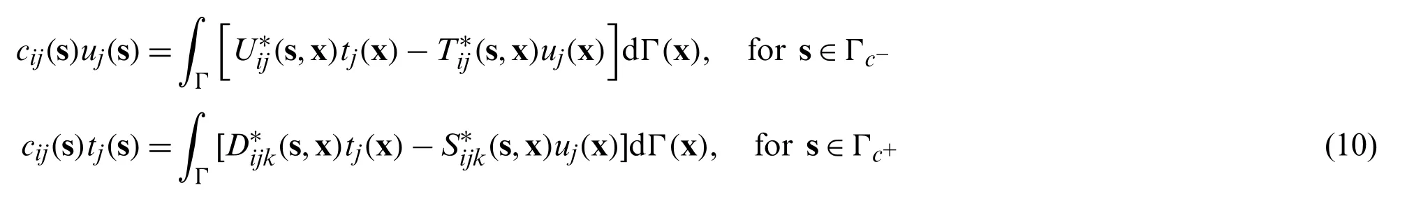
where s and x are the source point and the field point,respectively.andare the fundamental solutions of displacement boundary integral equations,andandare fundamental solutions of traction boundary integral equations(Appendix A).cij(s)denotes the jump term and equals 0.5δijfor smooth boundaries.

4.2 IGABEM for Fracture Mechanics

As a powerful geometric modeling technique,NURBS is the industrial standard of CAD and also central to isogeometric analysis.Given a knot vectorΞ=[ξ0,ξ1,...,ξm],which is a nondecreasing set of coordinates in parametric space,a B-spline basis function is defined as follows:

wherendenotes the order of basis functions andξthe parametric coordinate.As an extension of B-splines,NURBS basis function is written as

whereRi,p(ξ)is the NURBS basis function andwithe weight.A NURBS curve can be constructed by linear combination of NURBS basis functions and the associated coefficients

where x stands for the Cartesian coordinate of a point andξis its parametric coordinate.Pirepresents the Cartesian coordinates of control points in the physical space.

In IGABEM,NURBS are used not only for building geometries but also discretizing the boundary integral equations.Hence,the displacement and traction around the boundary can be expressed piecewisely as a linear combination of the NURBS basis function and the nodal parameters,

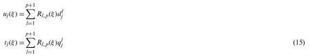
By substituting Eq.(15)into the boundary integral equation(10),we can get the following discretization formulation of Eq.(10)

The boundary element method involves weakly singular,strongly singular and hyper singular integrals,which have to be addressed carefully.For this purpose,the subtraction of singularity technique is used,whose implementation details can be seen in[50].After solving the governing linear equations of IGABEM,we can obtain the displacement and traction field around the boundary.Then,we are able to evaluate the stress intensity factors(SIFs)withMintegral[54]and predict the crack propagation direction with maximum hoop stress criterion[55].See Appendix B for details.

5 Numerical Examples

In the following examples,the input random variables are supposed to follow the Gaussian distribution with the expectation being 0.5 and the standard deviation being 0.033.The sampling method for Gaussian distribution function used in this paper is to select sample points in the interval[E−3D,E+3D].It is noted that only the problems with a single random input variable are considered in the present paper.The application of the method for the problems with multidimensional random input variables will be investigated in the future.

5.1 Inclined Center Crack Problem

A plate model with an inclined center crack under remote biaxial tension is considered in this section,as shown in Fig.3.The crack inclination angle isβ∈[0,π/2],edge lengthL=1,and crack length 2a=0.02.The loadσ0is applied in theX2-direction andλσ0is applied in theX1-direction,in whichλis the load ratio that varies from 0 to 1 andσ0=1.The Young’s modulus isE=1 and Poisson’s ratioυ=0.3.TheMintegral method is used for evaluating SIFs in this example.The analytical solution of the SIFs for the inclined center crack problem is available,as follows[56]:

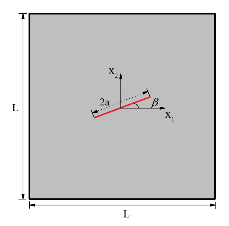
Figure 3:Structural model for an inclined center crack problem

The number of NURBS elements on the initial crack surface is set as 3,and the total DOFs is 86.We fix the crack angleβto beπ/4,and set the load ratioλas the input parameter.The response vector consists of 48 nodal displacements inX2-direction and two SIFs(K1andK2).Before MCs is carried out we firstly test the accuracy of ROM in evaluating SIFs.We select 21 sample points ofλthat are evenly distributed in the interval[0,1]to get the reduced bases of POD and interpolate the system responses with RBF.It is found that the values ofK1andK2computed by the numerical solution with ROM have a good agreement with the analytical solutions,as shown in Fig.4.

Figure 4:The variation of SIFs with the load ratio λ

Tab.1 lists the normalized values of SIFs(the values divided by the exact solution)calculated by the FOM with IGABEM and that by the ROM with POD-RBF.The normalized value ofK1changes slightly with the increase ofλ,while the normalized value ofK2increases steadily.Generally,both the results of the FOM and ROM are in good agreement with the analytical solutions.It is worth noting that the widthγof Gaussian kernel function has an important influence on the accuracy of RBF interpolation.According to the literature[57],the parameterγcan be determined via,whereNrepresents the number of samples andmrepresents the dimension of the random variable.

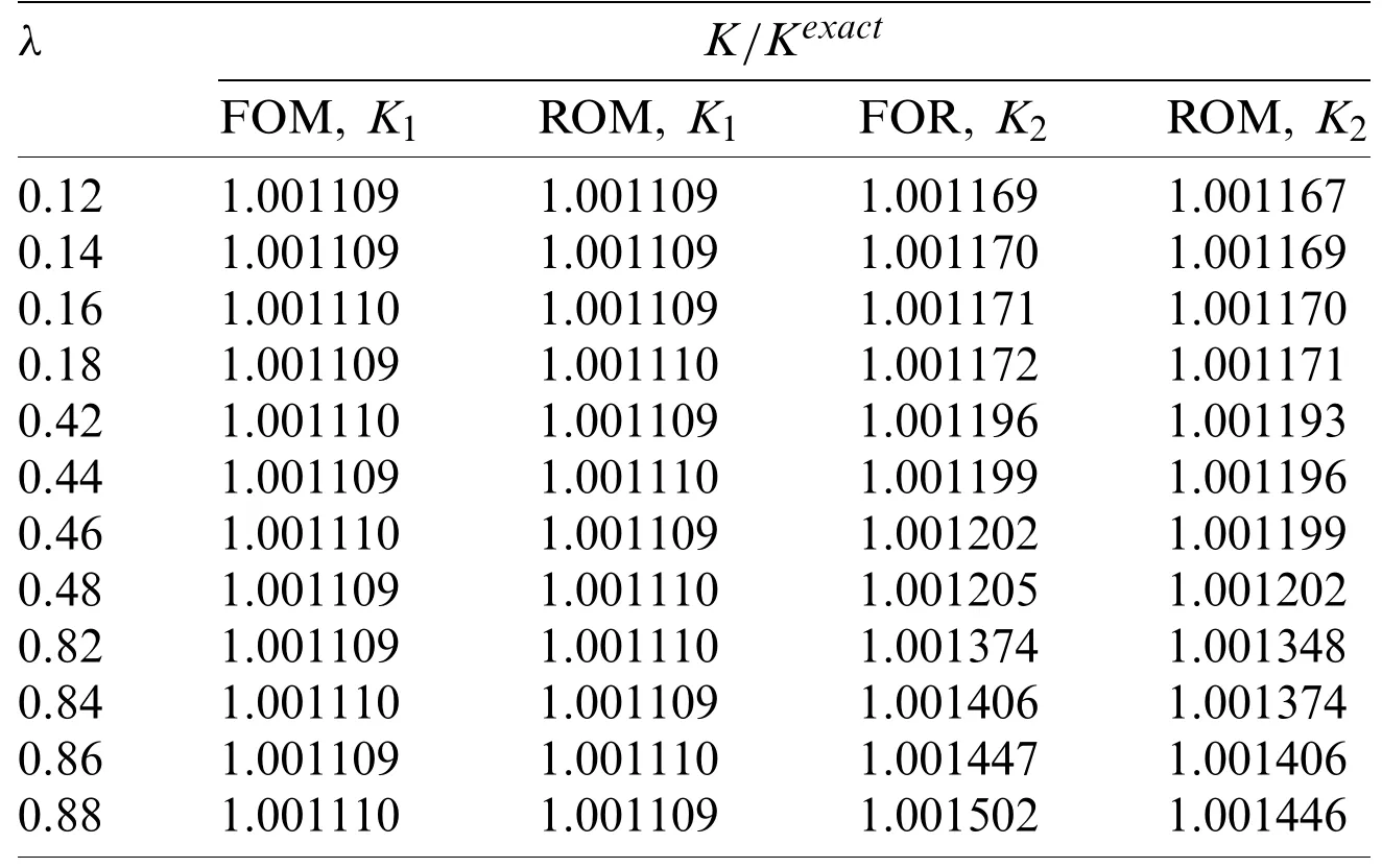
Table 1:Normalized results of the FOM and ROM

To investigate the influence of the sample size on the accuracy of ROM,we construct a vector,0.02,0.04,...,1,for different values ofλ.From the vector,20,40,60 and 80 samples are selected to form the reduced space,respectively,and the remaining points of the vector are used as the prediction points whose SIFs are computed with the ROM based on POD-RBF.We introduce R-squared method to quantify the accuracy of numerical results,as follows:

wherenis the total number of the predication points,the subscriptithei-th prediction point,yithe numerical value of the SIF,the analytical solution of the SIF,andthe average of the analytical solutions of the SIFs over these prediction points.The value of evaluation coefficientR2is between 0 and 1,which indicates the deviation of numerical solutions and the exact solutions.The closer its value is to 1,the higher the accuracy of the numerical result is.As shown in Tab.2,the evaluation coefficientR2gradually increases with the sample number.When the sample number is 80,the evaluation coefficientR2is 1.000,suggesting that the result of ROM is consistent with the analytical solution.It is also noted thatR2=0.859 when the sample size is 20,so a good accuracy can still be reached with moderate sample size.

Table 2:Comparison of the results of four different schemes

Next,we conduct MCs to evaluate the expectation and standard deviation of stress intensity factors.The following three different schemes are adopted for comparison.

1.Stochastic fracture analysis with MCs using FOM is conducted based on 51 samples ofλthat are evenly distributed between 0 and 1.Correspondingly the system equations need to be solved with IGABEM 51 times.

2.We build the ROM with 10,20,30,and 40 samples,respectively,and then perform MCs using the 51 samples.In this case,the dimension of the matrixΣin Eq.(5)is selected as min(m,n).

3.Similar to Case 2,the MCs is performed with the ROM that is established with 10,20,30 and 40 samples,respectively.However,we will further decrease the number of the reduced bases of the ROM by truncating theΣmatrix by 10−0.22σmax.

As can be seen from Figs.5 and 6,when the number of samples for reduced-order modeling is small,the results of Cases 2 and 3 have large deviation from that of Case 1.However,with the increase of samples,the solutions of Cases 2 and 3 approach that of Case 1 rapidly.With 30 samples,the solutions of Cases 2 agree with Case 1 well,which demonstrates that the combination of POD and RBF can evaluate the expectation and standard deviation in stochastic analysis accurately.In addition,because the number of reduced bases in Case 3 is decreased,a larger error occurs compared to Case 2 although the computational time is further accelerated.Therefore,it is very important to select an appropriate order for the ROM based on POD-RBF to strike a balance between its accuracy and efficiency.

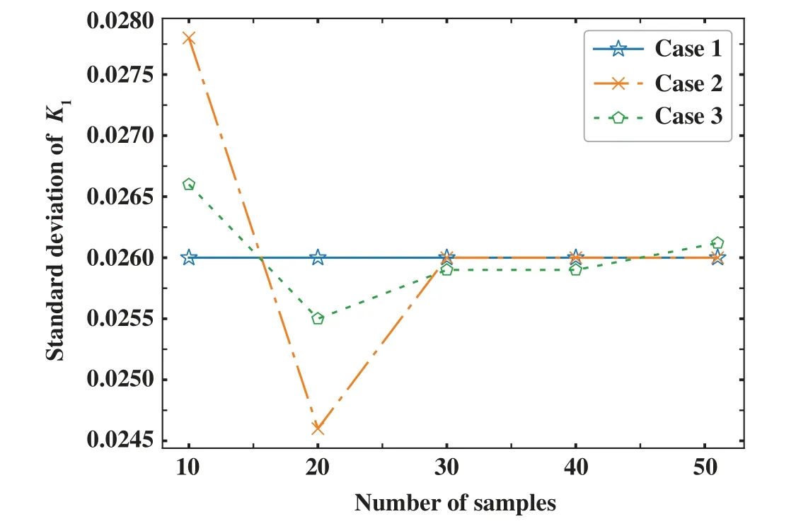
Figure 5:Standard deviation of K1

Now we fix the load ratioλat 0.5,and study the influence of the crack inclination angleβon the fracture analysis results.50 samples of the input parameterare used for Monte Carlo simulation,in which 25 samples are used for ROM.The SIFs in terms of different input variables are evaluated by POD-RBF and FOM,respectively(Fig.7).Tab.3 lists the values of the expectation and standard deviation of SIFs computed by MCs with FOM and ROM,respectively.It can be found from this table that the results of ROM and the FOM have good agreement to each other,which verifies the correctness and effectiveness of the algorithm.

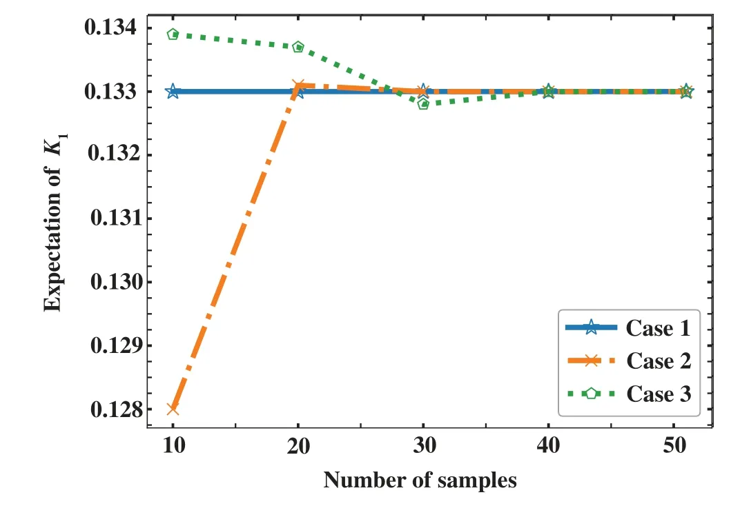
Figure 6:Expectation of K1

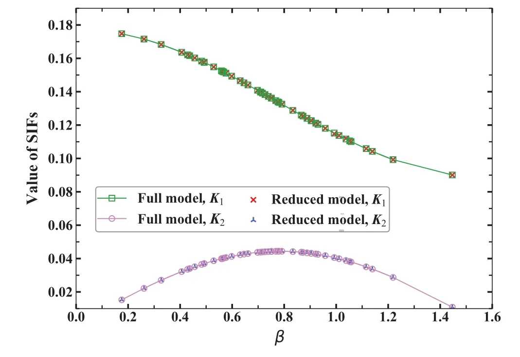
Figure 7:The value of SIFs obtained by using FOM and ROM

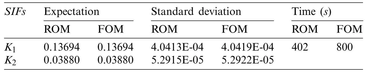
Table 3:Expectation,standard deviation and the corresponding calculation time with 50 samples

5.2 Cracks at Rivet Holes

In this section,we further test the performance of this algorithm using an example of a plate with two rivet holes,as shown in Fig.8.The Young’s modulus isE=1000 and Poisson’s ratioυ=0.3.The load isσy=1 andσx=0.The crack inclination angleθ=π/4,initial crack lengtha=0.1,and the number of NURBS elements on the crack surface is 3.

Figure 8:A plate with initial cracks emanating from the holes[58]

Suppose the radiusr∈(0.041,0.286)of the right circular hole is a random variable and follows a Gaussian distribution.Based on the FOM simulation with IGABEM,Fig.9 shows that theK1of the right crack increases significantly withr.We select 20 samples to construct ROM,and conduct MCs with 40 sampling points.Tab.4 shows the expectation,standard deviation and calculation time of MCs with FOM and ROM.It can be seen that the ROM leads to the results that are consistent with the FOM,and meanwhile reduces computational time.

Figure 9:The value of SIFs for two crack surface with the input parameter

Now we consider the influence of material parameter on displacement of cracks.The elastic modulusE∈(500,1500)is set as the input variable,which follows Gaussian distribution.51 samples are used for MCs,and 25 samples are used to construct the ROM based on POD and RBF.We choose the displacements of four collocation points on the crack surface as the response functions,whose coordinates are(2.91598244,2.49410744),(2.85147368,2.42959868),(2.08401756,2.50589256),and(2.14852632,2.57040132),respectively.Tab.5 shows the expectation,relative standard deviation(RSD)of the displacement inydirection and calculation time corresponding to reduced-order and full-order MCs,respectively.It can be found from Tab.5 that the stochastic analysis results of ROM are consistent with that of FOM.

Table 4:Expectation,standard deviation and calculation time

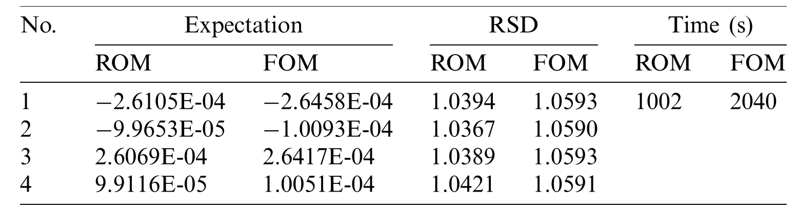
Table 5:Expectation,relative standard deviation and calculation time with MCs

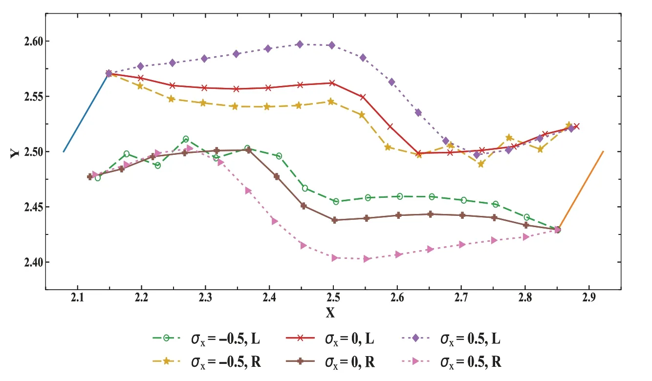
Figure 10:Crack propagation path under different loads

We also study how the crack propagation path is influenced by the input parameter ofσx.The crack propagation distance is fixed at 0.05 for each iteration step.A total of 16 steps are solved here.The path of crack propagation forσx=−0.5,0,0.5 is depicted in Fig.10.Supposing the input parameterσxfollows Gaussian distribution,we calculate the expectation and standard deviation of crack propagation path,which are represented by the coordinates of a series of crack tip positions.10 samples are employed for reduced-order modeling and and 20 samples for MCs.It can be seen from Tab.6 that the expectation and standard deviation of the crack extension path obtained from the ROM and that from the FOM have good consistency.It demonstrates the correctness and effectiveness of the stochastic analysis method proposed in this work.

Table 6:Expectation and standard deviation for Y coordinate of crack tip positions

6 Conclusion

The paper presents a novel framework for Monte Carlo simulation of multi-dimensional uncertainties of two-dimensional linear fracture mechanics.We use the NURBS to build the geometric model and discretize boundary integral equations.The IGABEM eliminates the repeatedly meshing procedure in uncertainty quantification,and retains the geometric exactness.The combination of POD and RBF accelerates the stochastic analysis and maintains good accuracy at low frequencies.In this work,the POD-RBF is used to approximate the structural response of a single random input variable.The method can also be extended to the problems with multidimensional random input variables,which will be investigated in the future.In addition,the present method will be applied to three dimensional problems and multi-physics coupling problems.

Funding Statement:The authors thank the financial support of National Natural Science Foundation of China(NSFC)under Grant(Nos.51904202,11902212,11901578).

Conflicts of Interest:The authors declare that they have no conflicts of interest to report regarding the present study.

Appendix A:Fundamental Solution

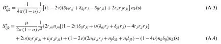
The fundamental solutions of displacement integral equationandare

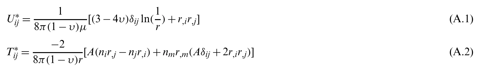
The fundamental solutions of traction integral equationandare

Appendix B:Evaluation of Stress Intensity Factors

TheMintegral based on theJintegral is an effective method to extract SIFs.TheJkintegral is defined as follows:

wherePkjis the Eshelby tensor,strain energy densityW=1/2σijεij.The center point of polar coordinate system is located at the crack tip.The limited integral boundaryΓεis an open circle with a center at the crack tip,as shown in Fig.A.1.

Figure A.1:J integral

Now,consider two independent equilibrium states of an elastically deformable object,the actual state(superscript‘1’)and the auxiliary state(superscript‘2’).Superimpose these two equilibrium states into one equilibrium state.It is assumed that the crack surface is flat in a sufficiently small radius of the contour circle.The conservation law can be reduced to the path-independentJintegral along an arbitrary pathΓεenclosing the crack tip located at the origin of the coordinates.Thus,theJintegral of the superposition state can be expressed as

Rearranging Eq.(B.2)into the following formulas:

where

withW(1,2)being the mutual potential energy density of the elastic body.

TheJintegral under two states can be expressed as a function associated withK,as follows:

Upon substitution of Eq.(B.3)into(B.5),we can obtain new expression of theMintegral,as follows:

TheMintegral shown in Eqs.(B.4)and(B.6)only involves interaction terms,which can be directly used to solve the mixed mode crack problem of linear elastic solids.

After SIFs are calculated,the direction of crack propagation can be determined by the maximum hoop stress criterion,the discriminant equation is as follows:

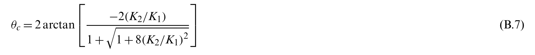
whereθcis the direction of crack propagation,in which the hoop stress is maximum.It can be seen that the accuracy of crack propagation simulation is mainly determined byK2/K1.