Aur´elien Decelle and Cyril Furtlehner

1Departamento de F´ısica T´eorica I,Universidad Complutense,28040 Madrid,Spain

2TAU team INRIA Saclay&LISN Universit´e Paris Saclay,Orsay 91405,France

Keywords: restricted Boltzmann machine(RBM),machine learning,statistical physics

1. Introduction

During the last decade,machine learning has experienced a rapid development,both in everyday life with the incredible success of image recognition used in various applications,and in research[1,2]where many different communities are now involved. This common effort involves fundamental aspects such as why it works or how to build new architectures and at the same time a search for new applications of machine learning to other fields,like for instance improving biomedical images segmentation[3]or detecting automatically phase transitions in physical systems.[4]Machine learning classical tasks are divided into at least two big categories: supervised and unsupervised learning (putting aside reinforcement learning and the more recently introduced approach of self-supervised learning). Supervised learning consists in learning a specific task — for instance recognizing an object on an image or a word in a speech — by giving the machine a set of samples together with the correct answer and correcting the prediction of the machine by minimizing a well-design and easy computable loss function.Unsupervised learning consists in learning a representation of the data given an explicit or implicit probability distribution,hence adjusting a likelihood function on the data. In this latter case,no label is assigned to the data and the result depends thus solely on the structure of the considered model and of the dataset.

In this review, we are interested in a particular model: the restricted Boltzmann machine (RBM). Originally called Harmonium[5]or product of experts,[6]RBMs were designed[7]to perform unsupervised tasks even though they can also be used to accomplish supervised learning in some sense. RBMs are part of what is called generative models which aim to learn a latent representation of the data in order to later be used to generate statistically similar new data—but different from those of the training set. There are Markov random fields(or Ising model for physicists),that were designed as a way to automatically interpret an image using a parallel architecture including a direct encoding of the probability of each“hypothesis”(latent description of a small portion of an image). Later on, RBMs started to take an important role in the machine learning(ML)community, when a simple learning algorithm introduced by Hinton et al.,[6]the contrastive divergence (CD), managed to learn a non-trivial dataset such as MNIST.[8]It was in the same period that RBMs became very popular in the ML community for its capability to pretrain deep neural networks (for instance deep auto-encoder),in a layer wise style. And,it was then showed that RBMs are universal approximator[9]of discrete distributions, that is, an arbitrary large RBM can approximate arbitrarily well any discrete distribution(which led to many rigorous results about the modelization mechanism of RBMs[10]).In addition,RBMs offer the possibility to be stacked to form a multi-layer generative model known as a deep Boltzmann machine(DBM).[11]In the more recent years,RBMs continued to attract scientific interest. Firstly because it can be used on continuous or discrete variable very easily.[12–15]Secondly, because the possible interpretations of the hidden nodes can be very useful.[16,17]Interestingly, in some cases, more elaborate methods such as GAN[18]are not working better.[19]Finally it can be used for other tasks as well, such as classification or representation learning.[20]Besides all these positive aspects, the learning process itself of the RBM remains poorly understood.The reasons are twofold: firstly,the gradient can be computed only in an approximated way as we will see;secondly,simple changes may have terrible impact on the learning or, messed up completely with the other meta-parameters. For instance making a naive change of variable in the MNIST dataset[21,22]can affect importantly the training performance(In MNIST,it is usual to consider binary variable{0,1}to describe the dataset. Taking instead {±1} naively will affect dramatically the learning of the RBM).In another example,varying the number of hidden nodes,while keeping the other mete-parameters fixed,will affect not only the representational power of the RBM but also the learning dynamics itself.

The statistical physics community,on its side,has a long tradition of studying inference and learning process with its own tools.Using idealized inference problems,it has managed in the past to shed light on the learning process of many ML models. For instance,in the Hopfield model,[23–26]a retrieval phase was characterized where the maximum number of patterns that can be retrieved can be expressed as a function of the temperature. Another example is the computation of the storage capacity of the Perceptron[27]on synthetic datasets.[28,29]In these approaches, the formalism of statistical physics explains the macroscopic behavior of the model in term of its position on a phase diagram in the large size limit.

From a purely technical point of view, the RBM can be seen for a physicist as a disordered Ising model on a bipartite graph. Yet,the difference with respect to the usual models that are studied in statistical physics is that the phase diagram of a trained RBM involves a highly non-trivial coupling matrix where the components are correlated as a result of the learning process. These dependencies make it non-trivial to adapt classical tools from statistical mechanics, such as the replica theory.[30]We will illustrate in this article how methods from statistical physics still have helped to characterize both the equilibrium phase of an idealized RBM where the coupling matrix has a structured spectrum, and how the learning dynamics can be analyzed in some specific regimes,both results being obtained with traditional mean-field approaches.

The paper is organized as follows. We will first give the definition of the RBM and review the typical learning algorithm used to train the model in Section 2,Then,in Section 3,we will review different types of RBMs by changing the prior on its variables and show explicit links with other models. In Section 4,we will review two approaches that characterize the phase diagram of the RBM and in particular its compositional phase,based on two different hypotheses over the structure of the parameters of the model. Finally, in Section 5, we will show some theoretical development helping to understand the formation of patterns inside the machine and how we can use the mean-field or TAP equations to learn the model.

2. Definition of the model and learning equations

2.1. Definition of the RBM

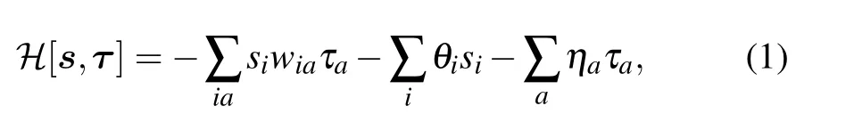
from which we define a Boltzmann distribution

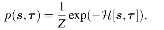
where Z is given by

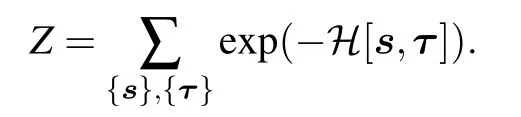
The structure of the RBM is presented in Fig.1 where the visible nodes are represented by black dots,the hidden nodes by red dots,and the weight matrix by blue dotted lines.

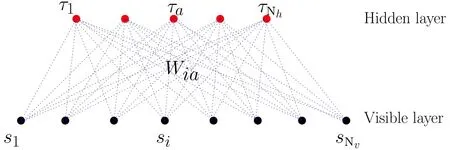
Fig.1. Bipartite structure of the RBM.

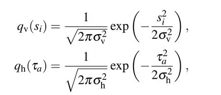
Historically,the RBM was first defined with binary{0,1}variables for both the visible and the hidden nodes in line with the sigmoid activation function of the perceptron, hence being directly intepretable as spin-glass model of statistical mechanics. A more general definition is considered here by introducing a prior distribution function for both the visible and hidden variables, allowing us to consider discrete or continuous variables. This generalization will allow us to see the links between RBMs and other well-known models of machine learning. From now on we will write all the equations for the generic case using the notations qv(σ)and qh(τ)to indicate an arbitrary choice of “prior” distribution. Averaging over the RBM measure corresponding to Hamiltonian(1)will then be denoted by

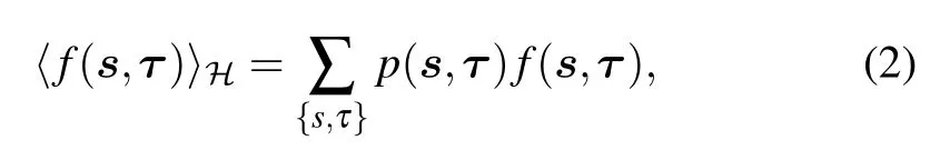
where Σ can represent both discrete sums or integrals and with the RBM distribution defined from now on as

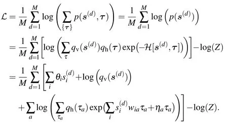
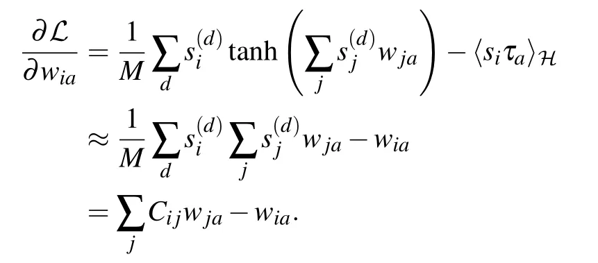
The gradient with respect to (w.r.t.) the different parameters will then take a simple form. Let us detail the computation of the gradient w.r.t. the weight matrix. By deriving the loglikelihood w.r.t. the weight matrix we get

where we have used the following notation:

The gradients for the biases(or magnetic fields)are

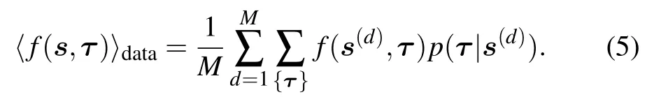
It is interesting to note that, in expression (4), the gradient is very similar to the one obtained in the traditional inverse Ising problem with the difference that in the inverse Ising problem the first term(sometimes coined“positive term”)depends only on the data,while for the RBM,we have a dependence on the model (yet simple to compute). Once the gradient is computed,the parameters of the model are updated in the following way:

where γ called the learning rate tunes the speed at which the parameters are updated in a given direction, the superscript t being the index of iteration. A continuous limit of the learning process can be formally defined by considering t real and replacing t+1 by t+dt,γ by γ dt and letting dt →0.

2.2. Stochastic gradient descent

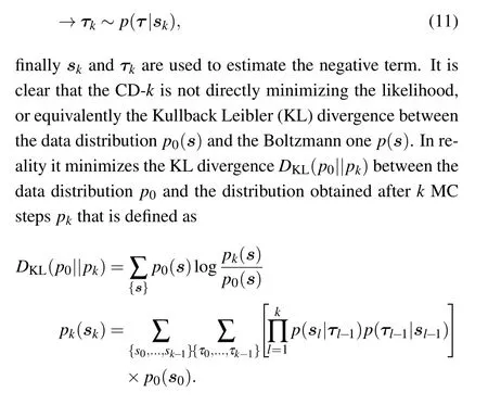
In Ref.[31]it is argued that this procedure is roughly equivalent to minimizing the following KL difference:

ℒCDk=DKL(p0||p)−DKL(pk||p),

up to an extra term considered to be small without much theoretical guaranty. The major drawback of this method is that the phase space of the learned RBM is never explored since we limit ourselves to k MC steps around the data configurations,therefore it can lead to estimate very poorly the probability distribution for configurations that lie“far away”from the dataset. A simple modification has been proposed to deal with this issue in Ref.[32]. The new algorithm is called persistent-CD (pCD) and consists of having again a set of parallel MC chains,but instead of using the dataset as initial condition,they are first initialized from random initial conditions and then the state of the chains is saved from one update of the parameters to the next one. In other words,the chains are initialized one time at the beginning of the learning and are then constantly updated a few MC steps further at each update of the parameters. In that case, it is no longer needed to have as many chains as the number of samples in the mini-batch even though in order to keep the statistical error comparable between the positive and the negative terms it should be of the same order. More details can be found in Ref.[32]about pCD and in Ref.[33]for a more general introduction to the learning behavior using MC.In Section 5,we will intend to understand some theoretical and numerical aspects of the RBMs learning process.

3. Overview of various RBM settings

Before investigating the learning behavior of RBMs, let us have a glimpse at various RBM settings and their relation to other models, by looking at common possible priors used for the visible and hidden nodes.

3.1. Gaussian–Gaussian RBM

The most elementary setting is the linear RBM, where both visible and hidden nodes have Gaussian priors:

Writing the distribution in this new basis we obtain

and we obtain a solution of the form

with

For δα≪1 we get a sigmoid type behavior

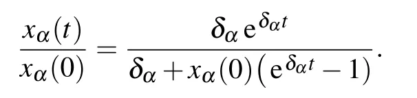
with

句中“天花乱坠”是佛教中的故事，语出《法华经·序品》。传说佛祖讲经，感动了天神，上天纷纷落下花来。后来，人们用“天花乱坠”来形容说话极其动听，但多指言语过分夸张，不切实际。杨译为 such a glowing picture，用“一幅美丽的图画”来指代“天花乱坠”，此翻译也算是意尽言至了，基本解决了译入语读者阅读时的理解问题。

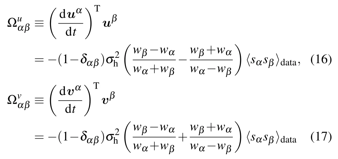
so that finally we get a dynamical system of the form

Note that at fixed x1and x2the dynamics of θ corresponds to the motion of a pendulum w.r.t the variable θ′=4θ shown in Fig.2.

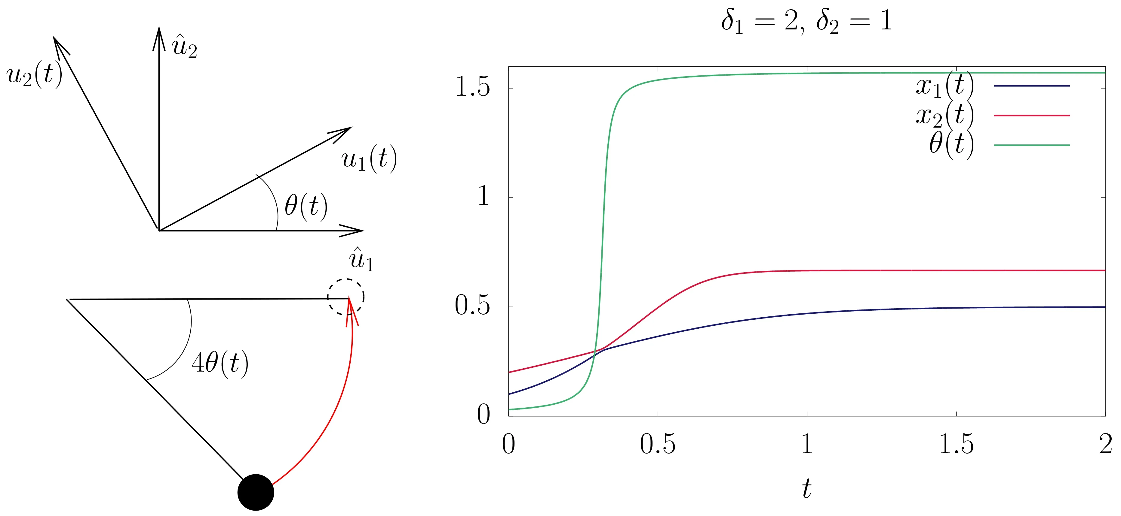
Fig.2. Angle between the reference basis given by the data and the moving one given by the RBM shown on the up left panel. Equivalence with the motion of a pendulum is indicated on the left bottom panel. Solution of Eqs.(18)–(20)of two coupled modes in the linear RBM(right panel).

3.2. Gaussian-spherical

To end up this section let us also mention that the finite size regime is amenable to an exact analysis when restricting the weight matrix spectrum to have the property of being doubly degenerated(see Ref.[40]for details).

3.3. Gaussian-softmax

The case of the Gaussian mixture if rarely viewed like that, fits actually perfectly the RBM architecture. Consider here the case of Gaussian visible nodes and a set of discrete{0,1}hidden variables with a constraint corresponding to the softmax activation function[42]

With this formulation,we indeed see that the conditional probability of activating a hidden node is a softmax function

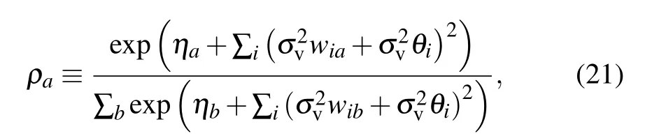
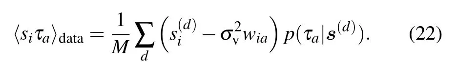
If we impose that the gradient is zero, doing now the “maximization”step,we obtain

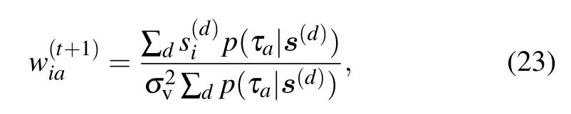
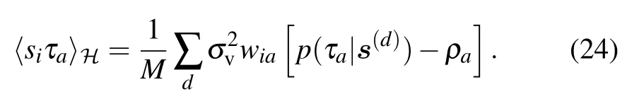
Interestingly,the threshold does not depend on the value of γ in that case,meaning that the instability is a generic property of the learning dynamics. The only change is the speed with which the instabilities will develop.

3.4. Bernoulli–Gaussian RBM

The next case is the Bernoulli–Gaussian RBM where we consider the following prior:

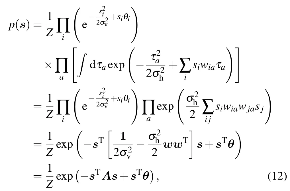
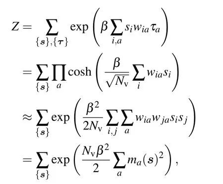
Again,a Gaussian prior implies that the activation function is Gaussian. It is interesting to consider this version of the RBM through its relation with the Hopfield model[23]was realized in Ref.[48]. Since the hidden variables are Gaussian they can be integrated out, which leads to a simple analytical form for the marginals of the visible variables. In some recent works,the opposite approach has been done, starting with a Hopfield model and expressing it as an RBM using the Hubbard–Stratonovitch(HS)transformation(expressing the exponential of a square as a Gaussian integral)to decouple the interactions between spins.[49,50]After integrating over the hidden nodes in Eq.(3),we end up with the following distribution:

We recognize a Hopfield model where the patterns are given by the weights wiaof the RBM and the effective coupling between two variables i and j is Jij=∑awiawja. We can also consider that the variances of the hidden nodes are related to the temperature of the model.

With this machine, it is also possible to impose a maximum rank in order to reduce the number of parameters needed to describe the dataset giving the possibility of a trade-off between a good description of the dataset and the number of parameters. This property has been used in Ref. [50] to find global patterns in protein foldings,using the RBM version of the Hopfield model with q discrete states.

3.5. Gaussian–Bernoulli RBM

At this point we now focus on models where the hidden layers will have a stronger impact. The integration of the hidden layer will not end up in a simple analytical form and therefore will make it difficult to understand the effect of the features and to characterize properly the learning dynamics. We first mention the Gaussian–Bernoulli case dealing with the following priors:

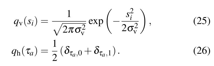
When using the discrete {0,1} variables, we obtain the sigmoid activation function for the hidden nodes

3.6. Bernoulli–Bernoulli RBM

The last model here is traditionally the one which is implied when speaking of RBM.In that case both the visible and hidden nodes are in{0,1}with the following priors:

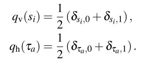
The activation functions are sigmoid functions, for both the hidden and visible nodes

In that case, the prior distribution has the advantage of not having any free parameter to be determined. In practice this model is used when dealing with a discrete dataset while the Gaussian–Benoulli is for continuous ones. This model can also be generalized to the case where the hidden nodes take more than two states, see Ref. [53] for more details on this approach.

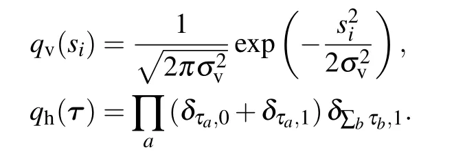
where we have defined the sigmoid function sig(x) = (1+exp(−x))−1. The r.h.s. of Eq.(29)is very close to the RELU activation function RELU(x)=max(0,x),hence showing that having all these replicas gives a similar activation function as RELU.In practice,it is not very efficient to have a large number of sigmoids for the training algorithm. An approximation is found by using the truncated Gaussian distribution. The average number of activated replica is then given by

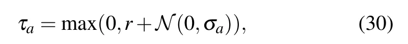
where now τais a RELU hidden node and σais the variance associated with the number of activated replicas for the hidden node a. Equation(30)can now be seen as an approximation of the truncated-Gaussian prior for the hidden nodes

In the following section, we will focus mainly on the Bernoulli–Bernoulli setting,its equilibrium phase diagram and its learning dynamics in the mean-field regime.

4. Phase diagram of the Bernoulli–Bernoulli RBM

4.1. Mean-field approach,the random-RBM

This MF approach to the macroscopic behavior of the RBM is based on statistical ensembles with iid elements of the weight matrix.Here,a random ensemble for the weight matrix is defined as follows. The weight matrix will be constructed. Now, each pattern is selected to be

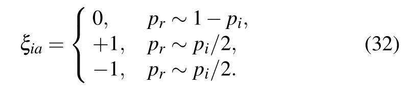
Using this definition, the degree of sparsity of the system is p=∑ipi/Nv. The term random-RBM was coined by Tubiana et al.,[58]but Agliari et al.[63,64]worked on a similar model although with a different theoretical approach. In particular,they computed the phase diagram in Ref.[57]. We start by reproducing here the argument of Agliari that was developed for the RBM with a finite number of patterns before switching to the replica computation done in Tubiana’s thesis.[60]

recovering the Hopfield model with a square inverse temperature, where we define the magnetization along the pattern a as . In Ref. [63], the authors considered a weight dilution as in Eq.(32)applied to the above binary–binary RBM,or equivalently to a Hopfield model with a rescaled temperature.It is important to mention that it is a different procedure than diluting the network itself, see Ref. [65] for more details on the other case. Having sparse patterns allows the network to retrieve more than one pattern at a time. In particular, global minima of the free energy can have an overlap with many patterns and locally stable states can be composed of a complex mixture of patterns. We reproduce below in Fig.3 the plot from Ref.[63]showing the overlap over three and six patterns in the(almost)zero temperature limit. We observe in the left panel that one pattern is fully retrieved when the dilution is low. Then,when increasing pi,more and more patterns are retrieved together until the system enters a paramagnetic phase at high dilution.

Fig.3. From Ref. [63]. Overlap with different patterns when varying the dilution factor p (named d on the figure) at low temperature. Left: a case with 3 patterns where we can observe how at small dilution,only one pattern is fully retrieved while the second and third ones appear for larger dilution.Right: a case with 6 patterns where the figure is zoomed in the high dilution region where the branching phenomenon is occurring and all the overlaps converge toward the same value.

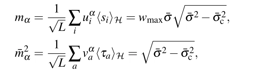
Replica approach of the random-RBMWe will now follow the approach of Tubiana et al.[60]and give more details on the derivation. This approach is based on a Bernoulli-RELU architecture giving the possibility to have continuous positive value for the hidden variables.

The characterization of the phase diagram is based on the determination of the free energy in thermodynamic limits.Given the weight ensemble(see Eq.(32)),the weight matrix is now made of independent and sparse elements.In this context,the replica analysis can be used to perform the quenched average. The replicated interaction term can be first easily computed and gives

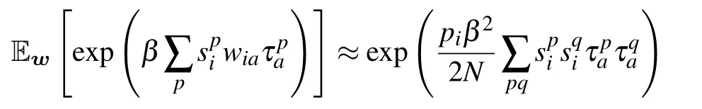
for the interaction term(ia). The interaction between the visible and hidden nodes can be decoupled using the HS transformation

introducing the spin-glass order parameter over the replicas(we denote by p,q,... the replica index)

• p<1,a ferromagnetic transition is found when imposing ˜L=1,where one pattern is recalled at a time.

• p<1, when all the hidden nodes are all weakly activated,a SG phase is found.

In this analysis, it is demonstrated that in the possible equilibrium behaviors of the random-RBM, an interesting phase mixing many patterns is present that characterizes in some way the efficient working regime of a learned RBM.It is of course a simplified case where the patterns are {±1} with a certain dilution factor. Now,the fact that there exists a family of weights where this phase exists is quite different from showing that the learning dynamics converges toward such a phase and how. In Tubiana’s thesis,a stability analysis of the different phases is done showing that for a range of parameters of the RBM, the compositional phase is indeed the dominant one. Then,a certain number of numerical results are provided on the MNIST dataset which tend to confirm that the behavior of the learned RBM looks similar to a“compositional phase”.It would therefore be of great interest to characterize the learning curve theoretically in order to understand how this phase is reached. It is also interesting to mention a recent work investigating the role of the diluted weights[66]during the learning in a RBM with one hidden node. In this article, it is shown that the proportion of diluted weights tends to vanish during the learning procedure. This might be a signal that when the number of hidden features is very low, the RBM automatically adjusts itself in the ferromagnetic phase described above,learning a global pattern of the dataset.

4.2. Mean-field approach using rank K weight matrix

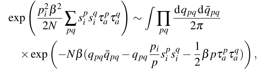
The difficulty with the RBM is to be able to study the phase diagram of the model without discarding the fact that during the learning, the weights wiabecome correlated between each others: starting from independently distributed wia,we can observe how the spectrum of the weight matrix is modified during the learning(see Fig.11 for instance). Classical approaches in statistical mechanics consider a set of independent weights,all identically distributed,before trying to compute the quenched free energy of the system by the replica trick(in few words,considering the quantity Znfor a given(integer)n,where Z is the partition function,for small n,we can develop Zn≈1+nlog(Z). The key point here is that it is generally possible to compute the quenched Znand then make a small n expansion). In the present case the hypothesis of independent weights cannot hold,as can be seen by looking at the spectrum of the weight matrix at the beginning of the learning and a few iterations later.The absorption of information by the machine prompts the development of strong correlations. This phenomenon is illustrated in Subsection 5.3 and in Fig.11. In order to understand how these eigenvalues affect the phase diagram of the system, it is reasonable to assume a particular statistical ensemble of the weight matrix of the form

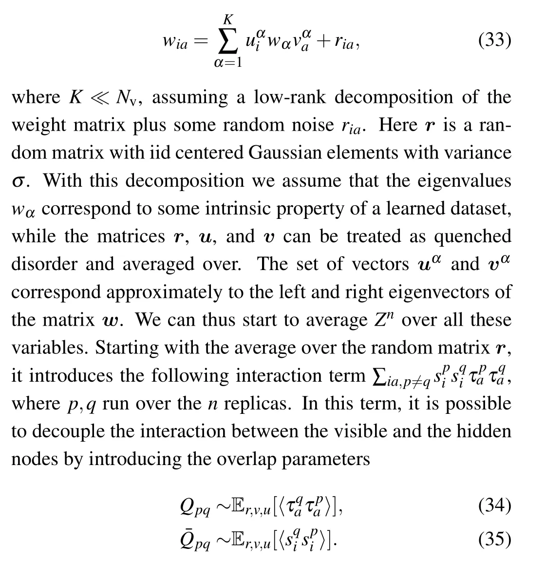
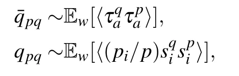
Then, the form of the weight matrix, Eq. (33), leads to the following change of variable:

we obtain two additional order parameters

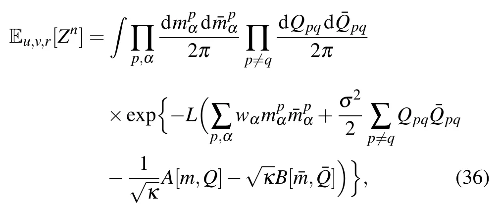
where E indicates an average over the variables that are in subscripts and κ =Nh/Nv. The quantities A and B are given by

where

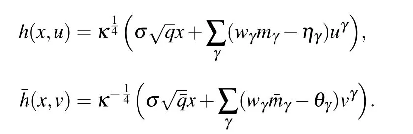
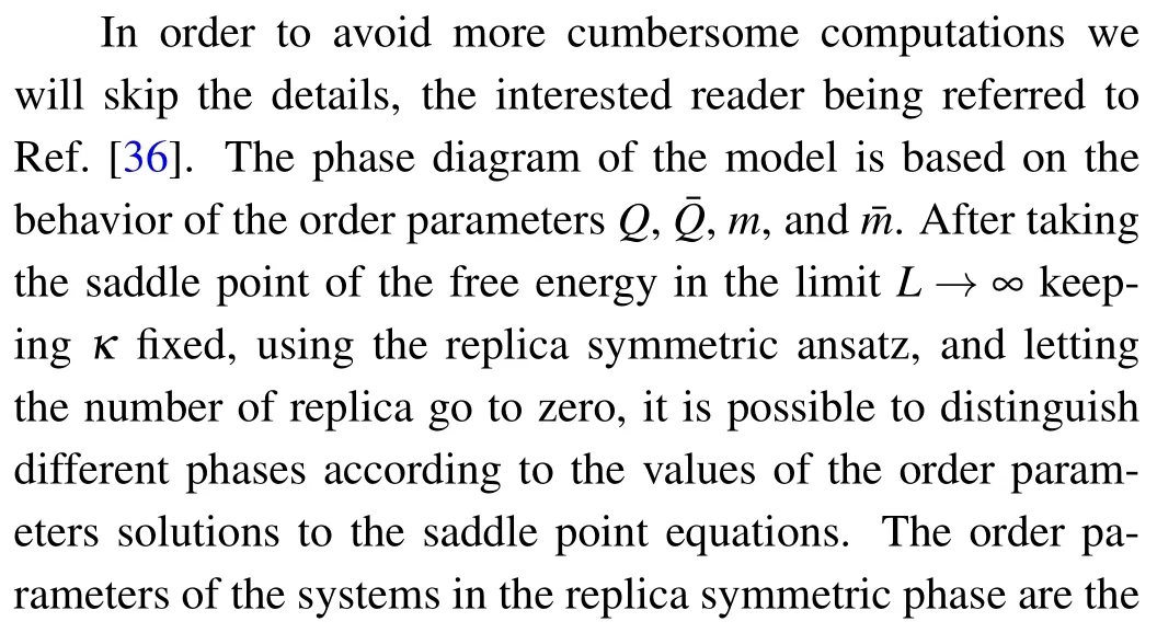
A first look at the equations for the magnetization over the mode α tells us that they correspond to the usual mean-field equations of the Sherrington–Kirkpatrick model[67]projected on the SVD decomposition of the weight matrix. The same is true for the overlap,with the difference that we have an overlap parameter for each layer. Analyzing these equations, we can distinguish three phases.

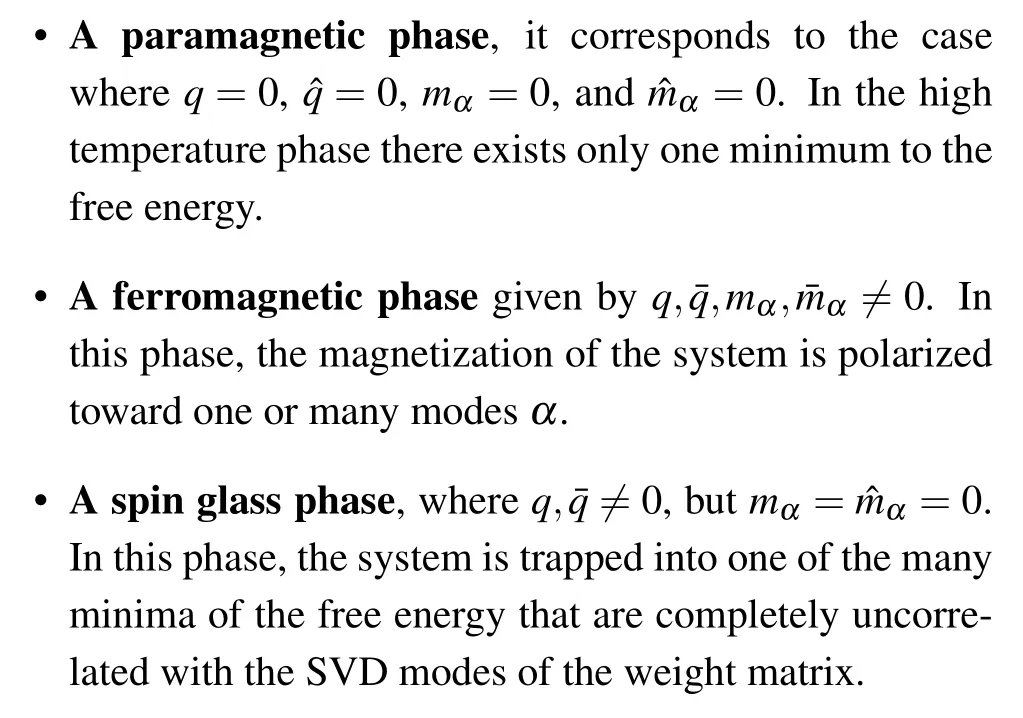
Fig.4. Left: the phase diagram of the model. The y-axis corresponds to the variance of the noise matrix,the x-axis to the value of the strongest mode of. We see that the ferromagnetic phase is characterized by having strong mode eigenvalues. In this phase,the system can behave either by recalling one eigenmode of or by composing many modes together(compositional phase). For the sake of completeness,we indicate the AT region where the replica symmetric solution is unstable,but for practical purpose we are not interested in this phase. Right: an example of a learning trajectory on the MNIST dataset (in red) and on a synthetic dataset (in blue). It shows that starting from the paramagnetic phase,the learning dynamics brings the system toward the ferromagnetic phase by learning a few strong modes.

• γ =0,e.g.,the Gaussian distribution. In this case,only the strongest mode is stable, and the weaker ones are unstable w.r.t. to the strongest one. Here, the system will condense along the strongest mode only.

• γ < 0, e.g., the uniform or the Bernoulli distribution.Here the weaker modes can be metastable if they are not“too far away”from the strongest one. However the system will condense only toward one mode.

• γ >0, e.g., a sparse Bernoulli, or the Laplace distribution. In this case, the strongest mode is unstable w.r.t.weaker ones, leaving the possibility to have condensation over many modes at the same time. This corresponds to a dual compositional phase, by reference to the terminology introduced in Ref. [58] which corresponds to combination of features instead of modes.

5. Learning RBM

5.1. Learning dynamics for exactly solvable RBMs

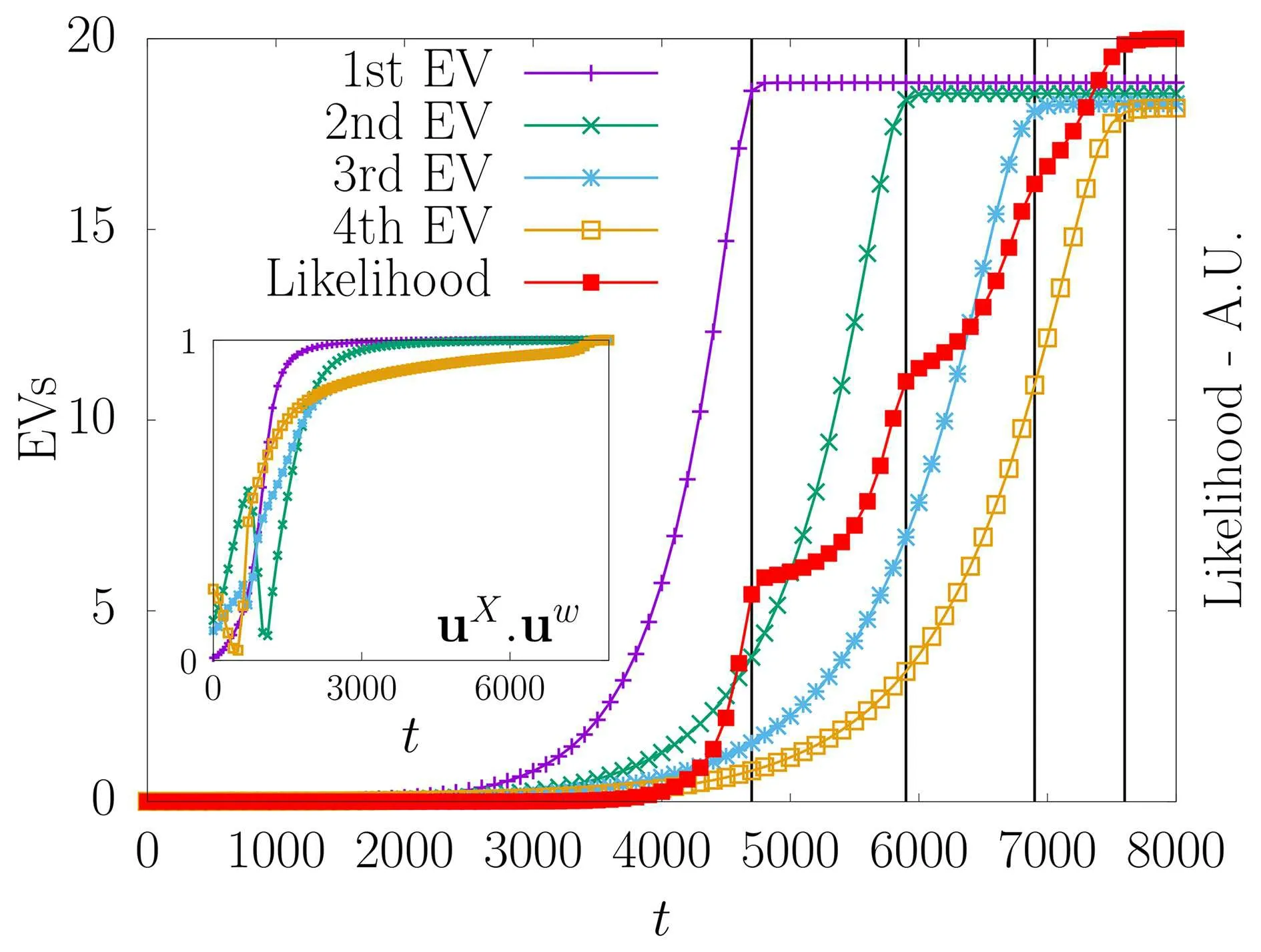
Fig.5. On this artificial dataset, we observe that eigenvalues that followare learned and reach the threshold indicated by Eq.(15). In the inset, the alignment of the first four principal directions of the matrix of the SVD of and of the dataset. In red, we observe that the likelihood function is increasing each time that a new mode emerges.

Fig.6. Left: the learning curves for the modes wα using an RBM with(Nv,Nh)=(100,100)learned on a synthetic dataset distributed in the neighborhood of a 20d ellipsoid embedded into a 100d space. Here the modes interact together: the weaker modes push the stronger ones higher, and they all accumulate at the top of the spectrum, as explained in Subsection 3.2. Right: a scatter plot projected on the first two SVD modes of the training(blue)and sampled data from the learned RBM(red)for a problem in dimension Nv =50 with two condensed modes. We can see that the learned matrix captures relevant directions and that the RBM generates data perfectly similar to the one of the training set.

5.2. Pattern formation in the 1D Ising chain

In a recent work,[69]the formation of features is studied analytically on a RBM with one hidden node. The training dataset is generated from a 1D Ising chain with a uniform coupling constant and periodic boundary conditions.The model used for generating the data has a translational symmetry which is exploited to solve the learning dynamics exactly.There is indeed available a closed form expression for the correlation function. Thanks to the translation invariance this depends only on the relative distance between the variables. Numerically,it is found that

• Using more hidden nodes (but still few), it is observed that each feature is peaked at different places and repels each other to encode the correlation patterns of the data.Again,the positions of the peaks diffuse with time even though some repulsive interaction seems to forbid them to cross. See Fig.7 taken from Ref.[69]illustrating this phenomenon.

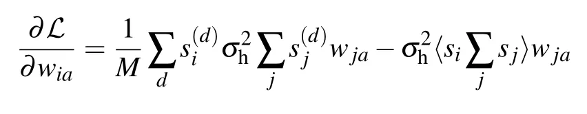
Now in Ref. [69], the author computed the gradient of a system with one hidden node

This expression can be developed up to the fourth order in w(and β),giving in the case of the 1D Ising chain

It is easy to identify in the first two terms the 1D discrete spatial diffusion. This equation can be cast into a spatial diffusion equation with additional term in the continuous time limit(see Ref. [69] for more details). From this small coupling expansion it is also possible to study the stationary solution in the one hidden node case and show that it is consistent with experimental results: it describes a peaked function decreasing rapidly as the distance from the center increases. An approximated weak coupling equation can also be derived in the case of two hidden units.In this case,an effective coupling between the two features vectors w1and w2is present and responsible for a repulsive interaction between the two peaks.

This illustrates nicely how the features learned by the RBM tend to describe local correlations between variables.In addition,these features diffuse over the whole system during the learning to restore the translational symmetry without crossing thanks to a repulsive interactions between them. In the next section,we will focus on the learning behavior on the MNIST dataset and see that in that case, the learned features similarly describe local correlations.

Fig.7. Left: figure from Ref.[69],the value of wi for each visible site of a RBM with 3 hidden nodes trained on the dataset of the 1D homogeneous Ising model with periodic boundary condition. We see three similarly peak shaped potentials with a decreasing magnitude of similar order for the three.Each peak intends to reproduce the correlation pattern around a central node,and therefore cannot reproduce the translational symmetry of the problem.Right: figure from Ref. [69], the position of the three peaks as a function of the number of training epochs. We observe that the peaks diffuse while repelling each others. The diffusion aims at reproducing the correlation patterns of the translational symmetry,while the repelling interaction ensures that two peaks will not overlap.

5.3. Pattern formation in MNIST:from SVD to ICA?

The pattern formation mechanism can be studied numerically on the MNIST dataset.MNIST[8]is one of the most used real dataset in machine learning, it contains 60000 images of black and white handwritten digits of 28×28 pixels,ranging from 0 to 9. The digits are about all the same size and are at the center of the image. They are illustrated in Fig.8.

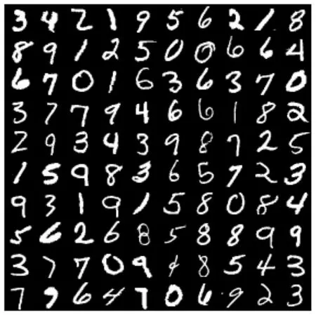
Fig.8. A subset of the MNIST dataset.

Additionally,at this stage of the learning the MC samples obtained from the RBM are typically prototypes: each sample is almost identical (or has a large overlap) with a learned feature. In fact, during the training, if we monitor samples at each epoch(keeping a low learning rate), we can see that the samples have a high overlap with one mode at the beginning,then later on with combinations of modes. To be more precise,we can distinguish different stages of the learning by inspecting the features, the produced samples, and the distance between the discretize features (taking the sign of each feature and computing the overlap). We illustrate these different stages in Fig.10.

To summarize we have identified the following stages:

• Stage 2: the RBM enters the ferromagnetic phase, the first strongest mode of the SVD is learned by all features, giving a high positive or negative overlap in the inter-features distances while the generated samples have a high overlap with the learned features.

• Stage 3: where many modes have emerged, but the learned features remain global and close to the modes of the dataset. The histogram of distances becomes much broader but the generated sample corresponds basically to the learned features with few variety. The RBM is in a pure Mattis phase analogous to the recall phase of the Hopfield model.

• Stage 4: finally,after a much longer period,we observe that the learned features are much alike an ICA decomposition while the distances between features are still centered in zero but with a much smaller variance. Finally the generated samples look very similar to the provided dataset. The RBM is in a compositional phase,both regarding the features and the modes (the dual one).

Fig.9. Left: the first 10 modes of the MNIST dataset(top)and the RBM(bottom)at the beginning of the learning. The similarity between most of them is clearly visible. Right: 100 random features of the RBM at the same moment of the learning. We can see that most features correspond to a mode of the dataset when comparing with the left-top panel.

Fig.10. The column represents respectively (i) the first hundred learned features, (ii) the histogram of distances between the binarized features:W±1 =sign(W), and (iii) 100 samples generated from the learned RBM. The first row corresponds to the beginning of the learning when only one feature is learned. Looking at the histogram,we see that most of the features have a high overlap. Also,the MC samples are all similar to the learned features. On the second row, the RBM has learned many features, and therefore the histogram is wider but still centered at zero. The MC sampling however is only capable of reproducing one of the learned features. On the last row the learning is much more advanced. The features tend to be very localized and the samples correspond now to digits.

Fig.11. (a)Singular values distribution of the initial random matrix compared to the Marchenko–Pastur law. (b)As the training proceeds we observe singular values passing above the threshold set by the Marchenko–Pastur law.(c)Distribution of the singular values after a long training:the Marchenko–Pastur distribution has disappeared and been replaced by a fat tailed distribution of eigenvalues mainly spreading above threshold and a peak of belowthreshold singular values near zero. The distribution of eigenvalues does not get close to any standard random matrix ensemble spectrum.

In future works,it could be interesting to understand the mechanism leading to the localization of the features,in particular whether this is related to some specific tail distribution of the weight matrix spectrum. An aspect of RBMs completely absent from the previous description of the learning process is the behavior of the biases associated to the hidden nodes.These are very important since they determine the threshold above which the features are activated and their learning dynamics is quite intertwined with the modes dynamics. This aspect of the learning could be worth studying especially to improve present learning algorithms.

5.4. Learning RBM using TAP equations

The difficulty of learning an RBM comes as already said from the negative term which requires to compute the thermal average of correlations between a visible and hidden nodes.In particular, when the machine starts to learn many modes,it becomes more and more difficult to estimate this term correctly using Monte–Carlo methods due to the eventually large relaxation time. In addition, to get a precise measurement, it is necessary to get many statistically independent samples in order to reduce the statistical error.

In this section we will derive the mean-field selfconsistent equations that can be used to approximate the negative term by using a high-temperature expansion of the Boltzmann measure. We illustrate the method showing the result of Gabri´e et al.[71]where an RBM has been trained by using the TAP equations. An interesting derivation using a variational approach in the case of the Gaussian–Bernoulli case has also been done in Ref.[72].

High-temperature(Plefka)expansionWe review here a famous approach using a high-temperature expansion of the system in order to compute the mean-field magnetization.This method is both very simple to implement and also provides a way to approximate the free energy of the system in the weak couplings regime. Recent successful approaches[73,74]showed how it is possible to train an RBM using these meanfield equations. For this subsection,we will use{±1}binary variables for simplicity.

For the Ising model, it is well-known that the (naive)mean-field (nMF) approximation can be written as a set of self-consistent equations on the magnetizations, and the associated approximation of the free energy can be computed as a function of these magnetizations

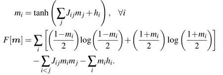
These equations can be translated directly to the case of the RBM, with the only need to specify clearly which variables are the visible and hidden ones. One gets the following:

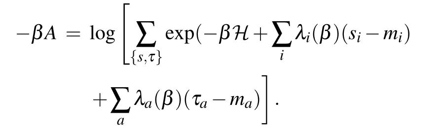
Using this expression,we can follow[77]and compute the magnetization in the infinite temperature limit of the following free energy:

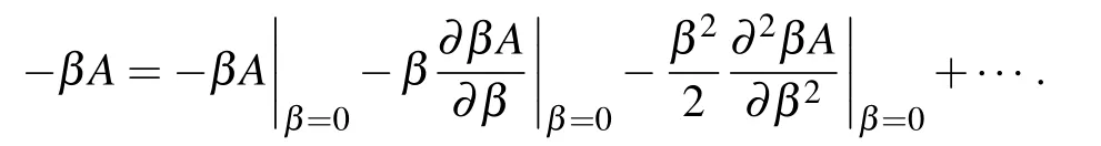
With our Hamiltonian, we can compute the first and second orders easily

where we have used the following identities for the second order computation:

As show in Ref. [73], the expansion can be easily extended to the third order without a big computational cost due to the particular topology of the RBM.Deriving the free energy obtained at this order w.r.t.the magnetization,we obtain the selfconsistent set of equations defining the TAP equations for the RBM

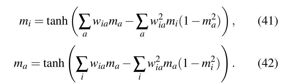
Hence, a solution of the TAP equations should satisfy Eqs. (41) and (42) and give us at the same time the approximated free energy associated to this solution

We can now use these mean-field equations to learn the RBM.First,we need to take into account the fact that many solutions to Eqs.(41)and(42)exist,each one with a given value of the free energy.Hence,the partition function can be approximated by

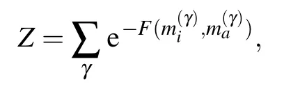
where the sum runs over all the possible solutions to the meanfield equations (41) and (42), weighted by the free energy given in Eq. (43). Using this approximation in the computation of the likelihood we obtain the following gradient:

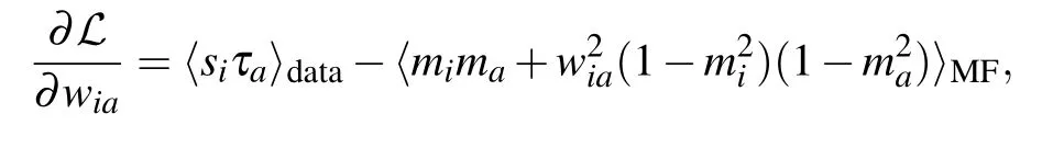
where

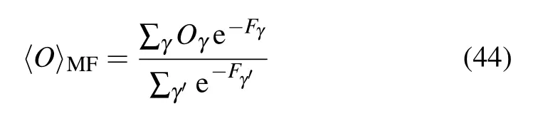
corresponds to the model average over all the solutions of the mean-field equations. We can see here a notable difference with the approach developed in Ref.[73]. In their work,Gabri´e et al. runs the sums over all obtained fixed points from the mean-field equations divided by the number of the fixed points only. The risk is that if the mean-field equations converge toward a fixed point that is suboptimal (having a high free energy)or even spurious(being a a maximum of the free energy) the estimation of the negative term will be polluted by such fixed points. More details on the Plefka expansion on bipartite Ising model can be found in Ref.[78]. As a final remark,let us insist on the fact that,even if the convergence of the TAP equations is not guaranteed,problems of convergence are practically not met in the ferromagnetic phase.On the contrary,such problems occur quite often in the spin glass phase which we wish to avoid in the context of learning the RBM.

Experiment with TAP learningWe show here some results obtained on MNIST using the same parameters as above but with the mean-field approximation taken from Ref. [73].Here, the comparison is done using the persistent chain algorithm, where a set of MC chains is maintained all along the learning whenever using CD,nMF,or the TAP approximation(in the case of nMF or TAP, the chain is updated using the corresponding self-consistent equations),see Fig.12.

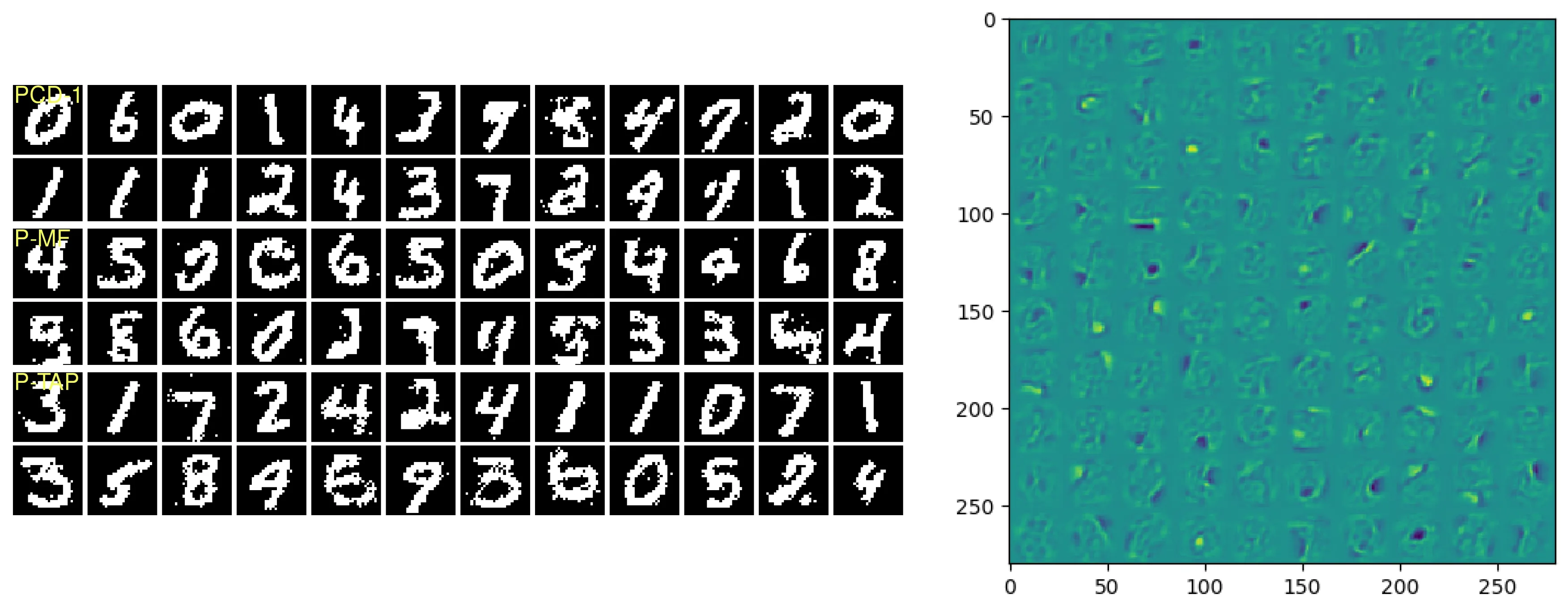
Fig.12. Top: figure taken from Ref.[73],the samples taken from the permanent chain at the end of the training of the RBM.The first two lines correspond to samples generated using PCD,the second two lines to samples obtained using the P-nMF approximation,and the last two,using P-TAP.Bottom: 100 features obtained after the training,we can see that they are qualitatively very similar to the ones obtained when training the RBM with P-TAP.

First we see that the samples generated by all the three methods are qualitatively similar. Second,the features learned are also qualitatively similar to the PCD case. Therefore, on the MNIST dataset the two machines are hardly distinguished by just looking at the generated samples and learned features,indicating that the MF/TAP approximation is working very well. It is also important to point out here that,the advantage of the mean-field approximation in that case does not rely on any speed up with regard to the learning procedure. But,more importantly,it provides complementary tools such as the fixed points as local maxima of the free energy and their associated free energy. For instance, in Ref. [79] an RBM is used as a prior distribution in the context of compressed sensing where the mean-field equations are used to infer equilibrium values of the variables. In Ref.[80],the RBM is used to reconstruct images from partial observations, again using the mean-field formulation to infer the states of the missing information.

5.5. Mean-field learning: ensemble average

In the approach developed in Ref.[36],using the statistical ensemble defined in Subsection 4.2 it is possible to have a mean-field estimate of the response functions involved in the gradient of the log-likelihood. For the response term on the data we get

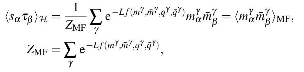
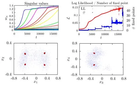
Fig.13. Top panel: Results for a RBM of size (Nv,Nh)=(1000,500) learned on a synthetic dataset of 104 samples having 20 clusters randomly located in a sub-manifold of dimension d =15. The learning curve for the eigemodes wα (left) and the associated likelihood function(right-red)together with the number of obtained fixed points at each epoch. We can see that,before the first eigenvalue is learned there is one single fixed point, then as modes are learned, the number of fixed points increases. Bottom panel: Results for an RBM of size(Nv,Nh)=(100,50)learned on a synthetic dataset of 104 samples having 11 clusters randomly defined a sub-manifold of dimension d=5. On the left,the scatter plot of the training data together with the position of the fixed points projected on the first two directions of the SVD of

We see again the different eigenvalues emerging one by one, and that each newly learned eigenvalue is triggering a jump of the likelihood together with a jump in the number of fixed points. At the end of the learning, the obtained meanfield fixed points are located at the center of each cluster of the dataset, as can be seen on the scatter plots. In Ref. [36], it is also shown that the behavior is qualitatively similar to what is routinely obtained when performing a standard learning based on PCD.

5.6. Other mean-field approach

6. Conclusion

With this review, we strive at showing that not only is RBM part of a hectic field of study,but it is also an intriguing puzzle with pieces which are missing in order to be able to understand the way these models can/could assimilate complex information/more complex information. While the black box nature of the learning process starts to fade away very slowly,there are still many key aspects that we do not understand or master for such simple models. We try to list interesting leads for the future.

Learning qualityDespite the fact that we are maximizing a likelihood function (which can not be computed) it is very hard to obtain a good indicator for comparing two learned RBMs. Even if many methods exist to compute the likelihood approximately[87,88]the obtained scores are in general not commented in regard to robust statistical analysis. If for very hard cases of image generation, it is easy to compare the results by eye inspection,there are no general method that manage to assess the quality of the samples in terms of how well the learned distribution reproduces the dataset distribution. Some recent work[89]introduced the notion of“ressemblance”and“privacy”that test the geometric repartition of the true data against the generated samples. This could be a first step defining scores according to different criteria (actually,this problem is not specific to the RBM but concerns actually most of the unsupervised learning models(GANs,VAEs,...).

The number of hidden nodesIt is striking that we are still unable to have a principled manner of deciding how many hidden nodes are necessary to learn datasets which are not too complex. For instance, on MNIST, it is possible to learn a machine with only 50 hidden nodes and it somehow manages to produce decent samples. The understanding on how much hidden nodes are necessary to reach a given sample quality is completely missing. In addition,the number of hidden nodes influences a lot the learning behavior of the machine,again in a way that is not fully understood.

The landscape of free energyWhen using statistical mechanics to understand RBMs,the natural question that comes in mind is about the landscape of free energy of the learned machine. It is easy to observe the mean-field fixed points obtained in the ferromagnetic phase and that they do correspond to prototypes of the dataset. Still, we do not know how these many fixed points are organized: are there low free energy paths relating them one from each others? do these paths define a network structure or instead separated clusters of low free energy?

The landscape of learned RBMsThis is a generic question in machine learning: what is the landscape of “good”learned machines in parameter space (here the weight matrix). For supervised tasks,some consensus seems to describe a space which is globally flat where all the good models are next to one another. However this is true for deep models, in the case of RBM,apart from the permutation symmetry of the hidden nodes,we have no clue about what this landscape looks like.

Link between the dataset and the learned featuresWe have seen that in the Gaussian–Gaussian case there is a direct link between the eigen-decomposition of the dataset and the learned features. However, for the non-linear model, we do not understand how the modes of the weight matrix are linked to the dataset,nor to the associated rotation matrices.