Long Fengyang Hu WuSheng Dong Yanfeng Yu Longfei

(School of Transportation, Southeast University, Nanjing 211189, China)

Abstract：To improve the applicability of the global pressure and temperature 2 wet (GPT2w) model in estimating the weighted mean temperature in China and adjacent areas, the error compensation technology based on the neural network was proposed, and a total of 374 800 meteorological profiles measured from 2006 to 2015 of 100 radiosonde stations distributed in China and adjacent areas were used to establish an enhanced empirical model for estimating the weighted mean temperature in this region. The data from 2016 to 2018 of the remaining 92 stations in this region was used to test the performance of the proposed model. Results show that the proposed model is about 14.9% better than the GPT2w model and about 7.6% better than the Bevis model with measured surface temperature in accuracy. The performance of the proposed model is significantly improved compared with the GPT2w model not only at different height ranges, but also in different months throughout the year. Moreover, the accuracy of the weighted mean temperature estimation is greatly improved in the northwestern region of China where the radiosonde stations are very rarely distributed. The proposed model shows a great application potential in the nationwide real-time ground-based global navigation satellite system (GNSS) water vapor remote sensing.

Key words：weighted mean temperature; GPT2w model; neural network; error compensation; GNSS meteorology

The water vapor is a highly variable component of the earth’s atmosphere, which plays a key role in the weather and climate systems even though it makes up only a small part of the atmosphere[1]. The precipitation water vapor (PWV) is an important parameter to study the variation of atmospheric water vapor, and the PWV retrieved by GNSS measurements has been widely used in the monitoring and prediction of various weather events such as short-term rainstorms, thunderstorms, strong winds and hurricanes etc[2-4]. The general principle of GNSS-PWV retrieval can be described as follows: When the electromagnetic signal emitted from a GNSS satellite travels through the neutral atmosphere, a certain delay will occur due to the effect of atmospheric refraction, and the part of delay caused by the water vapor in the atmosphere measured along the zenith direction is known as the tropospheric zenith wet delay (ZWD)[1,5]. The ZWD is approximately proportional to the water vapor content along the zenith direction and once the ZWD has been estimated from the GNSS measurements, the PWV can be calculated through a conversion coefficient. However, this conversion coefficient is a variable that depends on the weighted mean temperature, so it is important to obtain an accurate weighted mean temperature when converting the GNSS-ZWD to PWV[5]. Accurate weighted mean temperature at a specific location can be calculated via numerical integration by using the measured atmospheric profiles[1,6-7], but this method is not practical in the real-time or near real-time GNSS water vapor remote sensing, since it is difficult for general users to obtain accurate atmospheric profile data in time.

The precise modeling of the weighted mean temperature is an effective way to obtain accurate weighted mean temperature in real time. Many empirical models for predicting the weighted mean temperature have been developed in last decades, and they can be divided into two categories according to their applicable conditions. One is called the surface-meteorological weighted mean temperature (SMWMT) model. The SMWMT models are usually developed based on the relationship between the weighted mean temperature and surface meteorological elements such as surface temperature, pressure and water vapor pressure etc[8-9]. The other one is the non-meteorological weighted mean temperature (NMWMT) model, which refers to the models that can calculate weighted mean temperature without the measured meteorological elements[10-13]. The NMWMT models are usually less accurate than the SMWMT models, but they are more suitable for situations where meteorological elements are difficult to measure. Among the NMWMT models, the global pressure and temperature 2 wet (GPT2w) model is the most representative. It is a global blind model for estimating tropospheric delay, but it can also provide the empirical values of the temperature, pressure, water vapor pressure, and weighted mean temperature etc[14]. However, large systematic biases can be found for the GPT2w model when compared to the radiosonde data distributed in China and adjacent areas. The main reason is that the GPT2w model does not consider the impact of height differences between the target location and the gird points[7]. In this study, the model error compensation technology based on the neural network was proposed to enhance the performance of the GPT2w model in estimating weighted mean temperature in China and adjacent areas. The measured atmospheric profile data from radiosonde stations distributed in this region was used to establish an enhanced empirical model and verify its accuracy.

1 Determination of Weighted Mean Temperature

1.1 Weighted mean temperature calculated by numerical integration

During the GNSS water vapor remote sensing, the PWV can be calculated by multiplying the ZWD with a conversion coefficient, which is described as

(1)

wherek′2andk3are the atmospheric refraction constants;ρwis the density of liquid water;Rvis the specific gas constant of water vapor;Tmis the weighted mean temperature, which is a variable which can be calculated with the temperature and water vapor pressure along the zenith direction.

(2)

whereeandTare the water vapor pressure (in hPa) and absolute temperature (in K) of the atmosphere along the zenith direction;hsandhtare the height of the station and the tropopause, respectively.

However, it is not practical to calculate weighted mean temperature with the definition formula because the specific function expressions ofe/Tande/T2are usually unknown. However, the water vapor pressure and temperature at a series of sampling points along a vertical atmospheric profile can be measured, so the definition formula of the weighted mean temperature can be discretized into[8]

(3)

whereei,Ti,hiandei+1,Ti+1,hi+1are the water vapor pressure, temperature and height of two adjacent levels of a vertical atmospheric profile, respectively. The measured atmospheric profile data collected by the radiosonde and the reanalysis data from the numerical weather models (NWMs) can be used to calculate weighted mean temperature with this method.

1.2 Computing weighted mean temperature with the GPT2w model

The GPT2w model can be used to calculate the empirical value of weighted mean temperature. During the development of the GPT2w model, a trigonometric function was used to simulate the periodic variation characteristics of weighted mean temperature, which is described as

(4)

whereddenotes the day of the year;A0,A1,A2,B1,B2are the coefficients of the GPT2w model, and two sets of coefficients with the mesh resolution of 1°×1° and 5°×5° are provided by the global geodetic observing system (GGOS) atmosphere.

The GPT2w model is developed with the reanalysis products, and an unexpected large bias may occur in the weighted mean temperature estimates from the GPT2w model due to the differences between the reanalysis data and measured data[15]. Furthermore, the height differences between target location and grid points for interpolation were not considered, which leads to a significant negative bias for the GPT2w model in China and adjacent areas[7].

1.3 Computing weighted mean temperature with the Bevis model

The Bevis model is the earliest SMWMT model for weighted mean temperature calculation, and it is expressed as

Tm=aTs+b

(5)

whereTsis the measured surface temperature;aandbare the model coefficients, and they were fitted with the measured atmospheric profile data of 13 radiosonde stations distributed in North America[16]. However, the Bevis model also has significant limitations when applied to China and adjacent areas, since the variation characteristic of weighted mean temperature in this region may be different from that in North America.

2 Development of the Proposed Model

2.1 Data and study area

In general, the measured data collected by the sounding balloons is the closest to the actual situations, and the weighted mean temperature values derived from them are regarded as the most accurate one. They usually serve as the approximate true values for modeling and examining the performance of the weighted mean temperature models[15-17]. The radiosonde dataset is now available on the Integrated Global Radiosonde Archive (IGRA) (https://www.ncei.noaa.gov/data/igra/access/derived-por/)[6]. The dataset is organized according to the IGRA stations, and the atmospheric profile data of each station mainly consists of the meteorological elements at different heights along the zenith direction with a temporal resolution of 12 h, including the pressure, temperature and water vapor pressure etc.

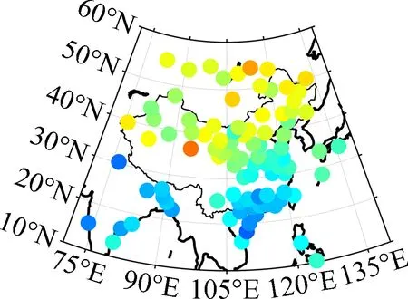
The study area chosen for this study is China and adjacent areas, where the data of 100 radiosonde stations measured from 2006 to 2015 was used for modeling and the remaining 92 stations for testing the performance of the proposed model. Fig.1 shows the distribution of radiosonde stations for modeling and testing. The stations for modeling should be almost evenly distributed to ensure the applicability of the proposed model.

2.2 Methodology

Several studies have discussed the systematic bias of the GPT2w model in estimating weighted mean temperature in China and adjacent areas, and the main reason is that the GPT2w model does not take the height of the target location into account[7,18]. In this work, we took the height and geographic coordinate of the station into account as input variables to establish an improved model. The proposed model is developed on the basis of the GPT2w model and makes use of the powerful multi-input nonlinear mapping capability of the artificial neural network (ANN)[19]. The model error compensation technology is also employed in the development of the proposed model. The flow diagram for establishing the model is shown in Fig.2.

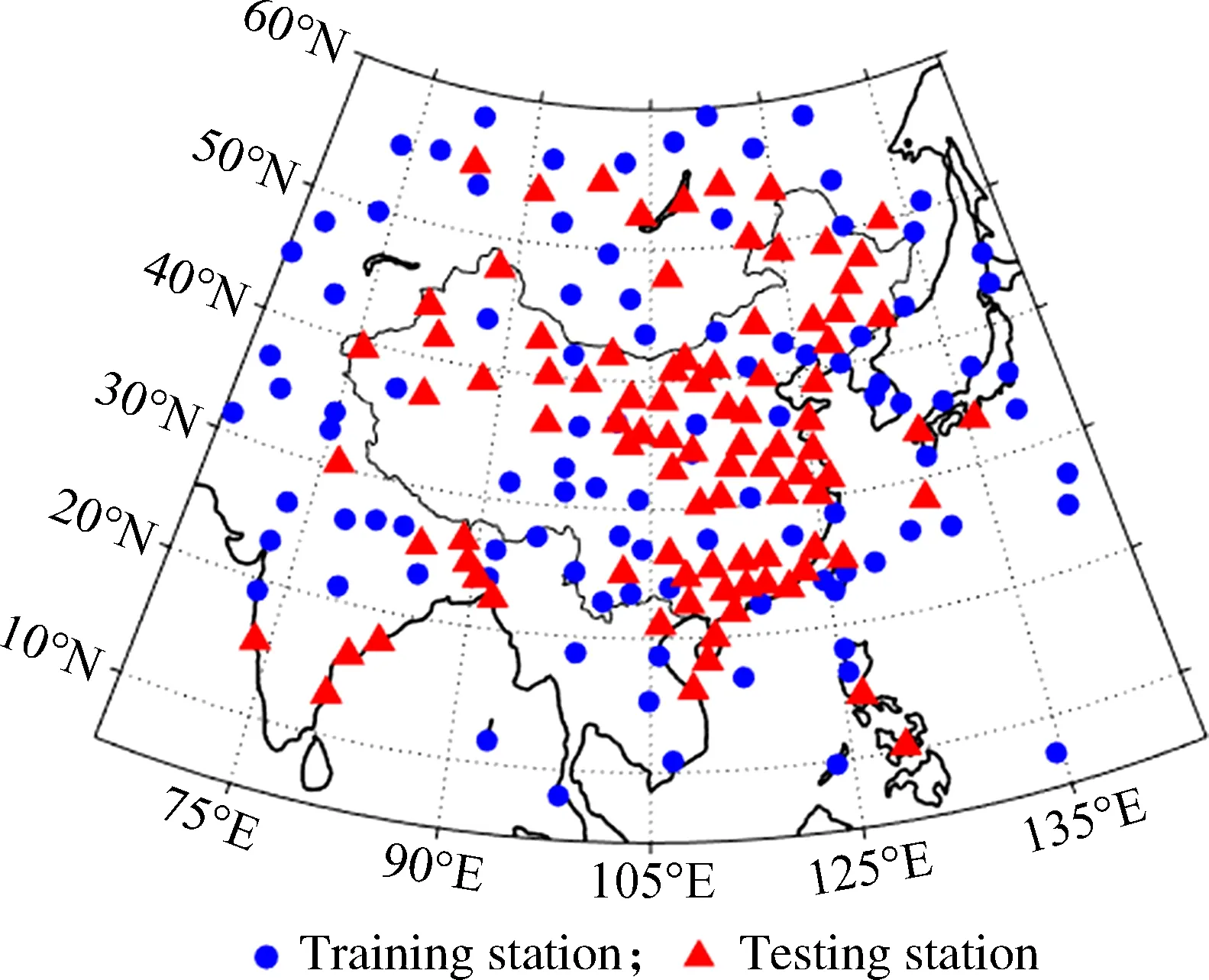
Fig.1 The distribution of radiosonde stations for modeling and testing

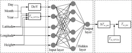
Fig.2 The flow diagram of establishing the model

Firstly, the empirical values of weighted mean temperature were calculated by the GPT2w model. Yao et al.[12]and Ding[17]suggested that the weighted mean temperatures derived from the GPT2w model should be corrected via a lapse rate factor in practice, so a constant lapse rate of -5.1 K/km was used in this study. The weighted mean temperature derived from the radiosonde data are usually regarded as the approximate true values, and they were used to calculate the residuals of weighted mean temperature estimates from the GPT2w model at this stage.

Secondly,the input and output variables were determined. The input variables include latitude (φ), longitude (λ), height (H) of the site, day of year (DoY) and the corrected value of weighted mean temperature determined by the GPT2w model (Tm_GPT2w). The output variable is the residual of the GPT2w model (ΔTm_GPT2w). The training samples should be normalized before use, and the normalized transformations were carried out by

(6)

wherexrandxnare the true value and normalized value, respectively;xmaxstands for the maximal value andxmindenotes the minimal value of each variable. We finally prepared a total of 374 800 samples for modeling.

Thirdly, the training mission of the neural network was carried out. A most popular learning algorithm, back-propagation (BP), was used for training. The optimal structure of an ANN model usually needs to be determined through a series of sensitivity tests, so the number of neurons in the hidden layer for each training mission was set to be 4 to 10, and each ANN structure was trained 10 times independently. The training results showed that when the number of neurons in the hidden layer is greater than 7, and the performance of the proposed model changes little and tends to be stable. In order to prevent the risk of overfitting, we determined a neural network structure of 5×7×1 as the core part of the proposed model.

Finally, we determined the optimal structure of the neural network and obtained the optimal weight and bias values. Users can just focus on how to use the final weight and bias values of the proposed model to calculate the weighted mean temperature instead of carrying out the training process again. For a single sample, the process of calculating weighted mean temperature with the proposed model can be described as

(7)

(8)

Tm_pre=Tm_GPT2w+ΔTm_pre

(9)

3 Results and Analysis

A total of 159 703 atmospheric profiles of 92 radiosonde stations measured from 2016 to 2018 were utilized to verify the performance of the GPT2w-NN model in comparison with the other two published models, the Bevis model and GPT2w model. The Bevis model is specified asTm=70.2+0.72Ts[9]. We considered using the Bevis model to calculate weighted mean temperature under two application conditions, one with the real surface temperature and the other without measured surface temperature. For the latter, the surface temperature derived from the GPT2w model was used. We called the Bevis models under these two application conditions the Bevis-R model and Bevis-V model, respectively. The bias and root-mean-square error (RMSE) were used to evaluate model accuracy.

3.1 Accuracies of different models tested by radiosonde data in the study area

We calculated the bias and RMSE of different models with the 159 703 testing samples, which are shown in Tab.1. The bias and RMSE of each testing station were also calculated.

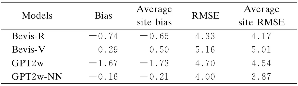
Tab.1 Bias and RMSE of different models K

One can see from Tab.1 that the GPT2w model shows the largest negative bias (-1.67 K), and significant systematic negative bias can be found for the GPT2w model. The Bevis-R model and Bevis-V model perform a little better in bias and no systematic bias has yet been found for them. The GPT2w-NN model, however, presents a much smaller bias (-0.16 K) and average site bias (-0.21 K), which verifies the good applicability of the proposed model in China and adjacent areas. From the aspect of RMSE, the Bevis-V model performs the worst that it has the largest RMSE and average site RMSE among all the competing models, but the Bevis-R model performs a little better than the GPT2w model. Significant improvement can be seen for the GPT2w-NN model that it is about 14.9% better than the GPT2w model, 22.5% better than the Bevis-V model and 7.6% better than the Bevis-R model in RMSE. The Bevis-R model belongs to the SMWMT model, but it is still inferior to the GPT2w-NN model in terms of both bias and RMSE.

3.2 Accuracy distribution for different models

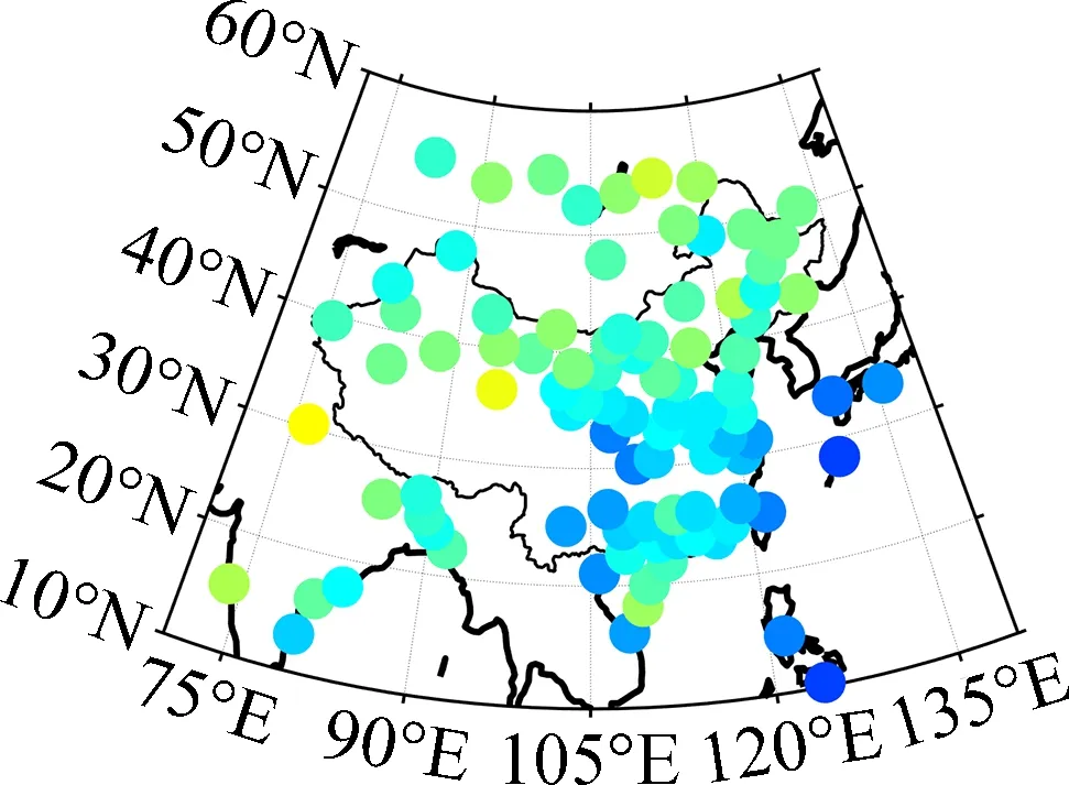
The distributions of bias and RMSE for each testing station are shown in Fig.3 and Fig.4, respectively.

(a) (b)

(a) (b)

One can see from Fig.3 that the Bevis-R model shows a large positive bias in the mid-latitude region (30°N-60°N) but large negative bias can be found in the low-latitude region (0°N-30°N), since the coefficients of the Bevis model were fitted by using the data in North America. Moreover, the geographic variations of the relationship between weighted mean temperature and surface temperature were not taken into account in the development of the Bevis model, which is another important reason for the significant regional differences of model accuracy. The positive bias of the Bevis-V model is much more significant in the northern part of the study area than the Bevis-R model, and the main reason is that the surface temperature estimated by the GPT2w model in this region is generally higher than the actual situation[19]. The GPT2w model shows large negative bias in the northwestern part of China than that in other regions, since the topography in the northwestern region is very complex and height fluctuates greatly, but the height differences between the testing stations and grid points were not considered. The biases of the GPT2w-NN model, however, are almost between -2.0 K and 2.0 K, and there is no remarkable bias for all the testing stations.

In terms of RMSE, the Bevis-R model and GPT2w model perform similarly, and a large RMSE can be found for them in the northern and western part of the study area. The accuracy of the GPT2w model is much lower than that of the Bevis-R model in the northwestern region of China, but in other regions, especially those stations at lower latitudes (around 20°N), the GPT2w model performs slightly better than the Bevis-R model. The reason is that the weighted mean temperature changes little in the regions near the equator, and the correlation of weighted mean temperature and surface temperature is weaker than that at higher latitudes[15]. A much larger RMSE can also be found for the Bevis-V model compared with the Bevis-R model. A common phenomenon for all the competing models is that the RMSEs in the north are larger than those in the southern part of the study area, which can be explained by the fact that the weighted mean temperature changes at higher latitudes are much larger than those at lower latitudes due to the solar radiation intensity[7]. It is remarkable that the GPT2w-NN model always performs the best of all the testing stations, and its model accuracy is significantly improved especially in the northwestern region of China where the radiosonde stations are rarely distributed.

3.3 Accuracies at different heights

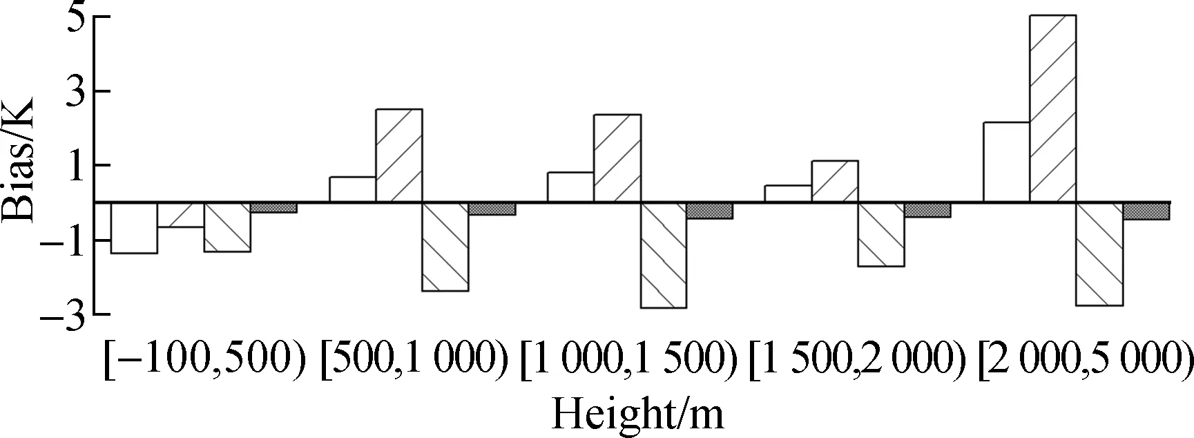
The greatest improvement of the GPT2w-NN model over the GPT2w model is that the height of the site was taken into account as the input variable, so the accuracies at different heights were discussed to verify the superiority of the proposed model. The testing samples were sorted into 5 groups according to the height, i.e., below 500 m, 500-1000 m, 1 000-1 500 m, 1 500-2 000 m and above 2000 m. The results are shown in Fig.5.

(a)

One can see from Fig.5 that the systematic negative biases for the GPT2w model are very remarkable at different heights, and the largest negative bias occurs at the heights from 500 m to 1 000 m. In contrast, a large negative bias can be seen for the Bevis-R model at the heights below 500 m, while a much larger positive bias is shown at the heights above 2 000 m. The Bevis-V model shows no significant bias at the heights below 500 m, but a large positive bias can be found as the height increases. The GPT2w-NN model, however, shows no significant bias at any height ranges, and the systematic negative bias caused by height differences has been eliminated effectively. In the aspect of RMSE, the GPT2w-NN model and Bevis-R model perform much better than the GPT2w model and Bevis-V model, especially at the heights above 500 m. The improvement of the GPT2w-NN model over the GPT2w model is significant, and it benefits not only from the consideration of the height as an input variable, but also from the use of local data.

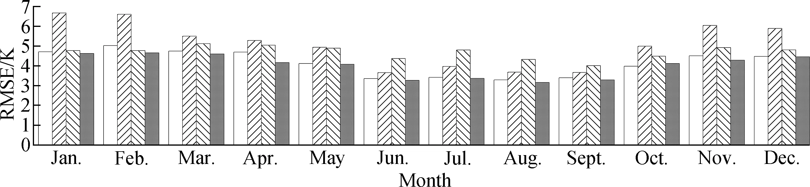
3.4 Seasonal accuracies of different models

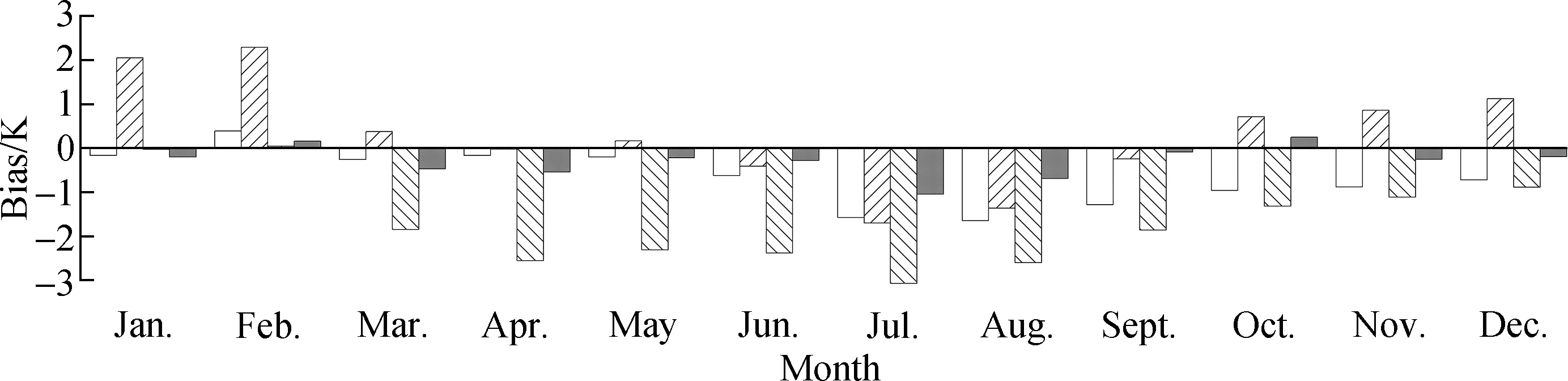
We further examined the seasonal performance of different models, and the bias and RMSE in different months are shown in Fig.6.

(a)

(b)

From Fig.6, significant negative biases can be found for the GPT2w model from March to December, and the biases are particularly large from April to August, nearly -3.0 K. Large negative biases can also be found in summer months for the Bevis-R model, but it shows smaller biases in other months. The Bevis-V model performs well in spring and autumn months, but significant positive biases are shown in winter, and large negative biases can be found during summer months. The GPT2w-NN model, however, shows smaller bias in each month compared with other competing models. A common phenomenon for all the competing models is that the biases in July and August are much larger than those in other months. We think the reason is that the study area is in the Northern Hemisphere, and the solar radiation is intense during summer, which leads to the larger weighted mean temperature than usual with variation characteristics that are not easy to be sufficiently captured by most of the competing models. In terms of RMSE, the Bevis-V model shows the largest RMSE from October to April, while the GPT2w model performs the poorest in the summer months. The Bevis-R model and GPT2w-NN model have similar performance, and the GPT2w-NN model has a slight advantage over the Bevis-R model in February and April. However, the GPT2w-NN model has more advantages over the Bevis-R model because it does not need any measured surface meteorological elements. Another common phenomenon for all the competing models is that the RMSE is the largest in the winter months but the smallest in summer months. It is mainly caused by the fact that the weighted mean temperature changes are great during winter and small during summer[20]. On the whole, the improvement of the GPT2w-NN model relative to the GPT2w model is significant, no matter whether from the perspectives of the seasonal or regional differences in model accuracy.

4 Conclusions

1) The GPT2w-NN model shows great improvement on the GPT2w model and Bevis model, which benefits from the powerful nonlinear mapping ability of neural networks. The neural network shows a powerful capability to capture the characteristics of relations between the weighted mean temperature and its associated factors in this study.

2) The improvement of the GPT2w-NN model also benefits from an important measure taken in this study, i.e., the height of the site was introduced as the input of the proposed model, which is the greatest difference between the GPT2w model and Bevis model.

3) The GPT2w-NN model takes the measured atmospheric profiles in China and adjacent areas as the data source, which is another reason why the GPT2w-NN model has been significantly improved compared with the GPT2w model.