DUAN Huo-yuan

(School of Mathematics and Statistics,Wuhan University,Wuhan 430072,China)

1 Introduction and Main Results

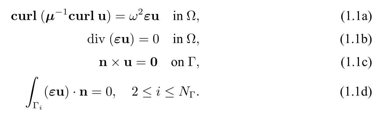
Let Ω⊂Rd,d=2,3,be a bounded Lipschitz domain,multiply connected.Let Γ denote the boundary of Ω,with a finit number of connected components Γi,1≤i≤NΓ,whereNΓis an integer number.Let Ω be occupied with discontinuous,anisotropic and inhomogeneous media ofµ(magnetic permeability)andε(electric permittivity).Let curl:=∇×and div:=∇·,with∇being the gradient operator,and let n be the outward unit normal vector to Γ.The Maxwell eigenproblem reads as follows:

Find eigenvalueω2>0 and eigenfunction u0 such that

We study the Lagrange finit element method for numerically solving the above problem(1.1).As is well-known,the Maxwell eigenproblem is usually solved by the so-called edge elements in the finit element discretization.The classic edge elements are Ne´de´lec elements([1,2]).Although the Lagrange elements have been the conventional and classical finit elements in the numerical solution of partial differential equations,they have been relatively not as popular as the edge elements in computational electromagnetism;as a matter of fact,in general meshes,some lower-order Lagrange elements such as the linear element have been widely recognized and well-known to generate spurious and incorrect discrete eigenmodes of the Maxwell eigenproblem.For this reason,there has been highly interesting in studying the Lagrange finit element method,typically for the Maxwell’s equations including the Maxwell eigenproblem,on how the Lagrange finit element method is used for obtaining correct and spurious-free approximations,cf.[3–13],and the references cited therein.However,all the existing Lagrange finit element methods in the literature that are valid for the correct numerical solutions of the Maxwell’s equations,and in particular,that are spurious-free and spectral-correct for the spectral approximations of the Maxwell eigenproblem,are based on some non-classical continuous or discrete variational formulations;all the discrete variational formulations have modifications different from the classical variational formulation(1.2).

The classical variational formulation for the Maxwell eigenproblem reads as follows:

Find(ω2>0,u0)∈R×H0(curl;Ω)such that for all v∈H0(curl;Ω),

The classical variational formulation(1.2)naturally incorporates all the constraints(1.1b)and(1.1d)of the Maxwell eigenproblem(1.1),while the perfect-conductor Dirichlet boundary condition is kept in the solution spaceH0(curl;Ω):={v∈(L2(Ω))d:curl v∈(L2(Ω))2d−3,n×v|Γ=0},where in two dimensions,t·v|Γ=0 with t being the counterclockwise unit tangential vector along Γ.Meanwhile,the classical variational formulation(1.2)is much simpler,particularly in implementations,than other variational formulations,and has been employed in practice.The well-known fact is that many of the Nédélec elements are spurious-free and spectral-correct for the classical variational formulation(1.2)in the finit element discretization.However,the issue has been open on whether the Lagrange elements could be spurious-free and spectral-correct for the classical variational formulation(1.2).Now,we have proven that all the Lagrange elements of any order are indeed spurious-free and spectral-correct for the classical variational formulation(1.2).The key and crucial property is the so-called discrete compactness,which is also the key and crucial property for those edge elements([14])which are spurious-free and spectral-correct for approximating the Maxwell eigenproblem with the use of the classical variational formulation(1.2).We have proven that all the Lagrange elements of any order hold the discrete compactness based on the classical variational formulation(1.2)in the finit element discretization.The meshes on which the Lagrange elements live may be required to be refine in some suitable manner for lower-order Lagrange elements and may be further required to have no singular vertices,edges,etc,for higher-order Lagrange elements.

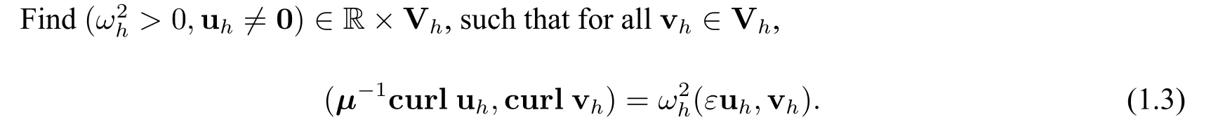
LetThdenote the shape-regular triangulations into triangles in two dimensions and tetrahedra in three dimensions.LetShdenote the triangulations of Ω into triangles in two dimensions and tetrahedra in three dimensions;Shis obtained possibly fromThby some suitable refinements Let Vh⊂H0(curl;Ω)∩(H1(Ω))ddenote the finit element space define with respect toSh.Each component of the finit element function vh∈VhisH1(Ω)-conforming,calledC0elements or Lagrange elements;all components of vhare independent of each other.The Lagrange finit element method based on the classical variational formulation(1.2)reads as follows:

For any element(triangle or tetrahedron)S∈Sh,letP‘(S)denote the usual space of polynomials of total degree less than or equal to‘≥1 for the integer‘.The Lagrange finit element space

is taken as either of the following Lagrange elements which include all Lagrange elements of any order:

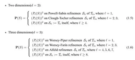
In the above,all the refinementShcan be found in the monograph[15].For the purpose of theoretical analysis,we introduce a scalar Hilbert space

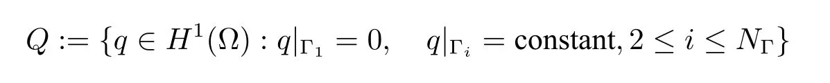
and letQh⊂Q∩H2(Ω)denote theC1element on the same meshesSh,which is a scalarH2(Ω)-conformingC1element.All the scalarH2(Ω)-conformingC1finit element spacesQhof lowerorder can be found in the monograph[15];higher-orderC1elements can also be similarly defined Defin the so-called discrete divergence-free space

Theorem 1.1[Discrete Compactness]Let Khbe defineby(1.7),while Vhis defineby(1.4),with either of P(S)given in the above(1.5)and(1.6).Then,Khis compactly imbedded into(L2(Ω))d,i.e.,the discrete compactness holds.

Remark 1.1In two dimensions,for Clough-Tocher refinemenShofTh,Theorem 1.1 has been essentially proven in[13],the firs theory and the firs result which have proved the discrete compactness of the Lagrange elementsof any orderon the Clough-Tocher meshes(of course,including the Lagrange elementsgiven by(1.5)for all).The theory in[13]is also straightforwardly applicable to the Lagrange elementsgiven by(1.5)for all.

2 Numerical Results

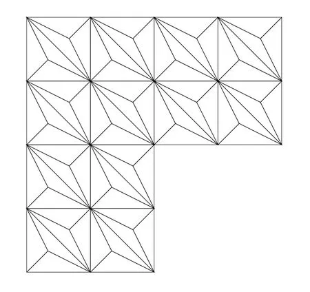
Figure 1 Clough-Tocher mesh

We report some numerical results using theP2quadratic element on the Clough-Tocher refine ment.The L-shaped domain(−1,1)2([0,1]×[−1,0]).The firs fve eigenvalues are available as follows(https://perso.univ-rennes1.fr/monique.dauge/benchmax.html):

The regularity for the eigenfunctions of the above fve eigenvalues are as follows:for any†>0,the 1rst Maxwell eigenfunction has(H2/3−†(Ω))2,the 2nd one belongs to(H4/3−†(Ω))2,the 3rd and 4th ones are analytic(exact value of the eigenvalueπ2=9.86960440108936),and the 5th one is(H4/3−†(Ω))2.The numerical results of the quadratic element on the Clough-Tocher mesh in Figure 1 are reported in Table 1.

AcknowledgementsThe numerical results are provided by Zhijie Du.

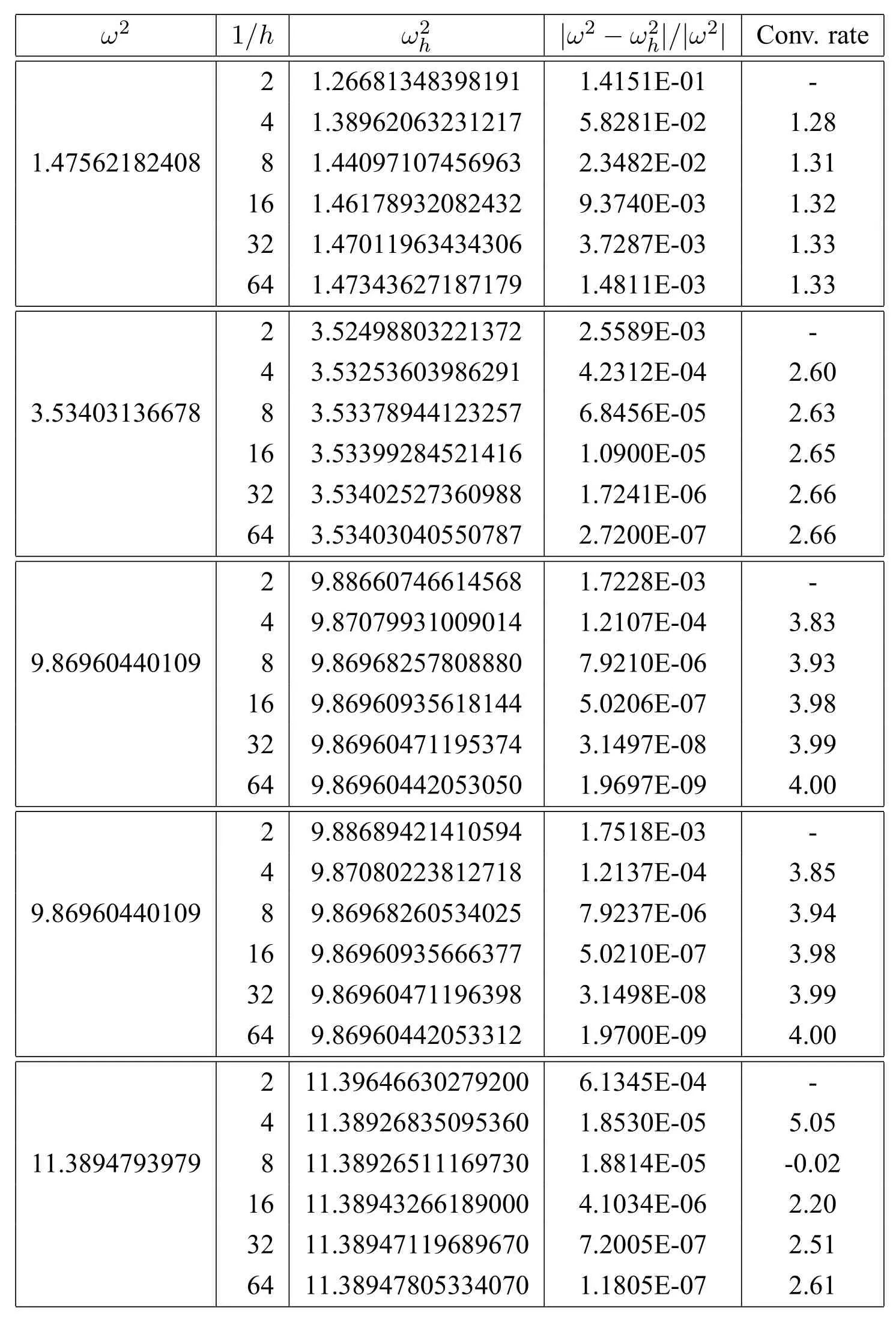
Table 1 Discrete eigenvalues and convergence rate in L-shaped domain