FU Gang, LIU Shan, LI Xiaodong, LI Pengyuan, and CHEN Lijia

Characteristics of Atmospheric Rivers over the East Asia in Middle Summers from 2001 to 2016

FU Gang1), 2), *, LIU Shan1), 3), 4), LI Xiaodong1), LI Pengyuan1), and CHEN Lijia1)

1) Department of Marine Meteorology, Ocean-Atmosphere Interaction and Climate Laboratory, Key Laboratory of Physical Oceanography, Ocean University of China, Qingdao 266100, China 2) Division of Oceanic Dynamics and Climate, Qingdao National Laboratory for Marine Science and Technology, Qingdao 266100, China 3) Qingdao Meteorological Bureau, Qingdao 266003, China 4) Qingdao Engineering Technology Research Center for Meteorological Disaster Prevention, Qingdao 266003, China

Atmospheric Rivers (ARs) are narrow and elongated water vapor belts in troposphere with meridional transport across the mid-latitudes towards high-latitudes. Compared with ARs occurred over the northeastern Pacific, the western coast of North America and Europe, the ARs over the East Asia have received less attention. In this paper, the characteristics of ARs which affected China in the area 20˚–60˚N, 95˚–165˚E in the middle summer season from 2001 to 2016 were investigated by using European Center for Medium-Range Weather Forecasts (ECMWF) ERA-Interim reanalysis data and Multi-functional Transport Satellites-1R (MTSAT-1R) infrared data. Totally, 134 ARs occurred during that period, and averagely 8.4 ARs occurred per year. Statistically, 101 ARs were in east-west orientation, and 33 ARs were in north-south orientation, which accounts for about 75% and 25%, respectively. Herein we report the occurrence number, duration time, intensity, length, width, ratio of length to width, and extension orientation of these ARs, which provide the basic information for those who have interest in ARs over the East Asia.

narrow and elongated water vapor belt; East Asia; middle summer season; Meiyu/Baiu front; characteristics of atmospheric rivers; infrared satellite data

1 Introduction

The term ‘atmospheric river’ (hereafter AR), refers to the ‘river in the sky’ (Kerr, 2006) with a narrow, elongated, synoptic jet of water vapor that plays important roles in the global water cycle and regional weather and hydrology (Guan and Waliser, 2015).A great number of previous studies (Zhu and Newell, 1998; Ralph, 2004; Ginemo, 2014; Nusbaumer and Noone, 2018) have indicated that ARs were one of the major causes of extreme precipitation and flooding in many regions around the world and contributed substantially to global poleward moisture transport.Zhu and Newell (1998) indicated that four or five atmospheric rivers in each hemisphere might carry the majority of the meridional water vapor fluxes over the globe. Gimeno(2014, p3) mentioned that ‘At 35˚N, it is estimated that 90% of the total meridional water vapor flux is due to ARs and that these structures cover about 10% of the total hemispheric circumference’.

Namias (1939) initially noticed the phenomenon of ‘river in the sky’. However, the concept of AR was firstly put forward by Newell(1992). By using European Center for Medium-Range Weather Forecasts (ECMWF) data, they documented the presence of the filamentary structure of water vapor belt, which had length several times of its width and might persist for several days. Newell(1992) termed this long (about 2000km), narrow (about 300km–500km) enhanced water vapor belt as the ‘tropospheric river’. Its maximum flow rate is close to that of the Amazon River in America, which is about 1.65×108kgs−1. Later, Zhu and Newell (1994) named this filamentary structure in atmospheric water vapor transport as ‘atmospheric river’.

By using the wind and relative humidity data in July from ECMWF containing the year 1991, 1994, and 1995, Zhu and Newell (1998) indicated that mean flow was mostly zonal in the tropics, with substantial meridional components between 35˚N and 55˚N in the North Atlantic and North Pacific, as well as south of Australia, southeast of South America, and in the southeast Pacific, but the transient perturbation flows were mostly poleward between 20˚–70˚S and 35˚–60˚N, particularly over the ocean.Ralph(2004) presented that a typical AR was positioned at the warm sector of the pre-cold-frontal region in a extratropical cyclone. The band of concentrated water vapor was in the narrow area at low levels, and strong low-level wind and high content of water vapor resulted in the intensive water vapor transport.

Bao(2006) investigated the moisture origin in ARs, and indicated that the water vapor in ARs had two origins. One was convergence of local moisture along the cold front, and the other was the water vapor transported to the poles (Bao, 2006). Before reaching extratropics, the majority of water vapor which was from south of 35˚N would re-circulate to the low latitudes (Knippertz and Wernli, 2010). Some previous studies of ARs suggested that the water vapor of ARs was from direct transportation from the tropics (Guan, 2010; Dettinger, 2011; Rutz, 2014). Within the weather systems over the ocean, the evaporation of water vapor, which was located behind the cold front, contributed significantly to the entire life cycle of cyclone. It was shown that as the cold front moved to the warm front cyclonically, which caused the warm sector to be narrower, local convergence of water vapor occurred along the cold front and was responsible for forming the plumes of enhanced water vapor (Dacre, 2015). ARs transported meridionally from tropics to the pole have directions from southwest to northeast normally. Hence, the east part of ocean, especially the west coast of North America and western European countries, were directly affected by landfalling ARs (Bao, 2006; Leung and Qian, 2009; Dettinger, 2011; Lavers, 2012; Dong, 2018).

Gimeno(2014) briefly reviewed the research history of AR, and pointed out that ‘ARs are narrow regions responsible for the majority of the poleward water vapor transport across the mid latitudes’. They mentioned that ‘ARs also had colloquial names, such as ‘Hawaiian firehose’ or ‘Pineapple Express’ (Lackmann and Gyakum, 1999), non-technical terms commonly used by forecasters to refer to ARs that connect tropical moisture near the Hawaiian Islands with the west coast of North America. Over the central United States ARs have been named the ‘Maya Express’ (Dirmeyer and Kinter, 2009).

Compared with the ARs over the Northeastern Pacific (Lackmann and Gyakum, 1999; Neiman, 2008, 2011; Ralph and Dettinger, 2011; Ralph, 2011, 2019; Waliser, 2012; Payne and Magnusdottir, 2014; Warner and Mass, 2015; Sellars, 2017), especially the extreme precipitation caused by ARs over California (Dettinger, 2011; Cordeira, 2013; Luo and Tung, 2015; Ralph, 2016) and ARs over the Europe (Lavers, 2011, 2012; Ramos, 2014; Gao and Leung, 2016), ARs that affect China have received less attention.

Chinais typically influenced by monsoon climate with cold and dry winters and the warm and wet summers. In summer, China is usually characterized by arainy season, commonly referred to as plum rain, which is caused by precipitation along a persistent atmospheric stationary front known as the Meiyu/Baiu front for nearly two months from the late spring to the early summer among China, Korea, and Japan. The rainy season usually ends when the sub- tropical high-pressure system becomes strong enough to push the Meiyu/Baiu front to the north of China. For a long time, the seasonal and long-term water scarcities had been one of the most serious threats to the north of China.

In this paper, we aim to investigate the characteristics of ARs over the East Asia which may affect China, and try to address the following questions: what are the characteristics, such as occurrence frequency, spatial-temporal scales of ARs over the East Asia in middle summer season? These questions are necessary and significant approaches towards much deeper understanding of ARs over the East Asia which may affect China. The rest of this paper is arranged as follows: The data and methodologywill be introduced in Section 2. Characteristics, such as the occurrence number, duration time, intensity, length, width, ratio of length to width of ARs over the East Asia which may affect China will be documentedin Section 3. Finally, concluding remarks will be given in Section 4.

2 Data and Methodology

2.1 Data Sources

In the present study, we used the European Centre for Medium-Range Weather Forecasts (ECWMF) global reanalysis (ERA-Interim) data with the spatial resolution of 0.5˚×0.5˚①ERA-Interim data are originally reduced Gaussian grid data with approximately uniform 79km spacing for surface and other grid-point fields. When we downloaded ERA-Interim data, they were regridded to spatial resolution of 0.5˚×0.5˚ already.. The study period is from 15 June to 31 July from 2001 to 2016, which covers the Meiyu/Baiu season in East Asia. Variables include geopotential height, air tem- perature, three-dimensional wind components,, and, specific humidity and relative humidity with 37 isobaric levels (1000, 975, 950, 925, 900, 875, 850, 825, 800, 775, 750, 700, 650, 600, 550, 500, 450, 400, 350, 300, 250, 225, 200, 175, 150, 125, 100, 70, 50, 30, 20, 10, 7, 5, 3, 2, and 1hPa) and 6-hourly temporal resolution (00, 06, 12, and 18 UTC). Multi-functional Transport Satellites-1R (MTSAT-1R) infrared data, which was supplied by Kochi University of Japan (http://weather.is.kochi-u.ac.jp/archive-e.html) from 2001 to 2016, are utilized to document the evolutionary processes of cloud systems. MTSAT-1R data are 1-hourly on horizontal resolution of 0.05˚×0.05˚ within the area of 20˚S–70˚N, 70˚–160˚E.

2.2 Method to Identify AR

The methodology we used in the present study is similar to the algorithm of moisture fluxes suggested by Zhu and Newell (1998) to diagnose the AR based on IVT mag- nitude. In the following, IVT is calculated:

Fig.1 shows the MTSAT-1R infrared satellite image at 00 UTC 20 July 2016 together with IVT distribution. It is found that a nearly NE-SW oriented cloud system occupied the east part of China mainland. The concentrated IVT contours with the maximum value of 1700kgm−1s−1coincide with the cloud system. This cloud system is an AR which deserves further investigation.

Fig.1 MTSAT-1R infrared satellite image at 00 UTC 20 July 2016 (shaded, bright temperature with the unit of ℃, 2℃ interval) together with IVT distribution (blue contours, 100kgm−1s−1 interval) and IVT=800kgm−1s−1 interval (red contour).

One of the challenges of investigating ARs is how to define the AR event (Sellars, 2017).In previous studies, the threshold values using IVT to quantify AR in different regions varied significantly by different researchers.Some researchers defined AR based on the 85th percentile of peak water moisture flux (Guan and Waliser, 2015; Waliser and Guan, 2017). Mahoney(2016) took 500kgm−1s−1as the threshold of the AR edge in southeast of the United States. By using JRA-55 data, Kamae(2017) calculated the climatology of monthly mean IVT field in June, July and August. They suggested an anomalous IVT threshold of 140kgm−1s−1to be used to detect AR-like water vapor belt over the northwestern Pacific. Kamae(personal communication, on 15 September 2018) also indicated that the IVT value around the central East China Sea (30˚N, 125˚E) could be obtained by plus anomalous IVT field 140kgm−1s−1with the monthly meanIVT field 600kgm−1s−1,, total IVT field 740kgm−1s−1.Employing ERA-2 reanalysis data during the period from 1980 to 2016, Sellars(2017) set a minimum threshold of IVT intensity at 750kgm−1s−1to be an AR. Their results showed the global regions where intense AR often existed in five areas,, off the coast of the Southeast United States, eastern China, eastern South America, off the southern tip of South Africa, and in the southeastern Pacific Ocean.

In summer season, there is a large amount of water vapor transport in the region of Asian monsoon. In the present study, we choose IVT threshold value 800kgm−1s−1to quantify AR based on the following considerations.

1) The focus period of the present study is from 15 June to 31 July, which covers the middle summer season in China. The Meiyu/Baiu front may contribute heavy precipitations in the south of China. Thus, it is reasonable to consider more abundant water vapor in the definition of AR than that in other seasons.

2) The AR with the same IVT intensity is more likely to cause extreme precipitation in regions with large topography variation. As in the north of China, the topography variation is not very pronounced, thus, it needs more water vapors in flatlands than that in mountainous area for extreme precipitation caused by ARs. Therefore, IVT threshold value of identifying AR should be greater than that of other regions with large topography variation. Thus in the present study, the 800kgm−1s−1threshold value, which is slightly greater than the threshold values suggested by Kamae (personal communication, 2018) and Sellars(2017), is selected to target only the extreme water vapor transport processes. Another supporting evidence of using 800kgm−1s−1IVT threshold in the present study might be Fig.1b in Guan and Waliser (2015), where the 85th percentile of summertime IVT is shown to be much larger over East Asian region compared to western US or Europe.

In the later analyses, the following principles must be followed:1) The water vapor band which affected China should be formed within the area of 20˚N–60˚N, 95˚E–165˚E with its maximum IVT value greater than 800kgm−1s−1. 2) The ratio of length to width of the water vapor band is not less than 2, and its duration time is longer than 12h. 3) Even if a water vapor belt is consisted of multiple connected parts, it is regarded as one united water vapor band.

Based on the aforementioned principles, all long and narrow water vapor bands whose maximum IVT value greater than 800kgm−1s−1were examined. Finally, for all water vapor bands which satisfy the selection criteria are defined as AR in the present study.

In the following, it is essential to illustrate how to calculate the length and width of AR. In Fig.2a, the arc line AA’ refers to the longest distance between any two points in the outmost edge of AR, which represents the length of AR. While the arc line BB’, which is perpendicular to arc line AA’, represents the width of AR. Suppose the latitude of point A is1, the longitude of point A is1, the latitude of point A’ is2, and the longitude of point A’ is2, the length of arc line AA’ is calculated as:

Here,=6371km is the radius of the earth. It is easy to calculate the length of arc line BB’ in a similar way.

Setting the southernmost point of line AA’ as the original point (shown in Fig.2b), if the direction of line AA’ (defined as the difference between these two latitudes) falls within area A or area D, then AR is in east-west orientation. If the direction of line AA’ falls within area B or area C, AR is in north-south orientation. The duration time of AR is set to be the period from its beginning to its end②Here, the ‘beginning’ is defined to be the ‘appearing time’ of contour of 800kgm−1s−1 IVT together with the ratio of length to width greater than 2. The ‘end’ is defined to be the ‘disappearing time’ of contour of 800kgm−1s−1 IVT, or the ratio of length to width less than 2.. The duration time, length, width, ratio of length to width, the maximum IVT value, and extension orientation which represents the characteristics of these ARs are documented from their beginnings to the ends. Detailed information of all 134 ARs is listed in the Appendix.

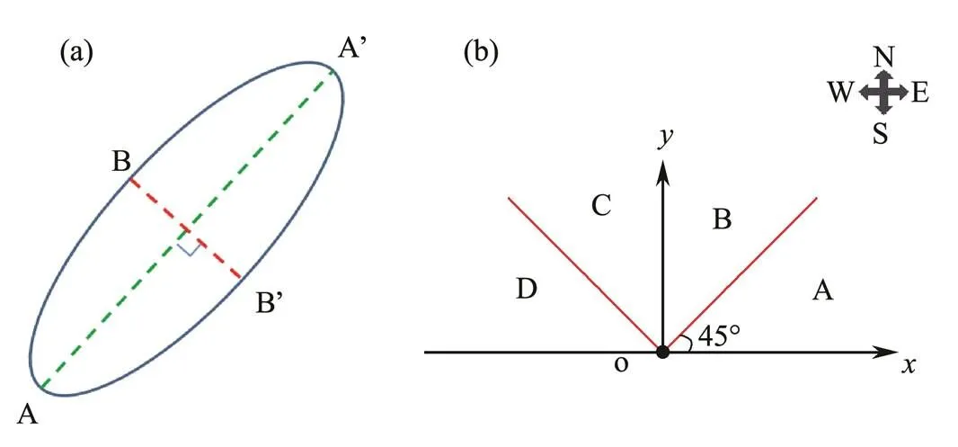
Fig.2 Schematic diagram for an ideal‘Atmospheric River’. (a) The length and width of an atmospheric river. Blue line represents the outmost edge of atmospheric river. Arc line AA’ represents the length of atmospheric river, and arc line BB’, which is perpendicular to line AA’, indicates the width of atmospheric river. (b) The orientation of atmospheric river. x-axis represents the east-west orientation, while the y-axis represents the north-south orientation.

3 Statistical Results

Based on the aforementioned principles, totally 134 fila- ment-shaped bands with enhanced water vapor flux were determined in the present study.

Fig.3 shows the occurrence yearthe occurrence of AR numbers over the East Asia during the period from 15 June to 31 July from 2001 to 2016. It is found that the numbers of AR in the year of 2004, 2005 and 2010 were all 10. In each summer, there are averagely 8.4 ARs over the East Asia. In 2009, the maximum numbers of AR were 11, while the minimum numbers of AR were 5 in 2015. The numbers of AR in different years varied significantly, with the mean value of 8.4 and the variance of 3.05.

In the present study, we used the maximum IVT value to represent the intensity of AR. As shown in Fig.4, the maximum value of IVT ranges from 800.1kgm−1s−1to 2400kgm−1s−1. Respectively, there are 33 ARs whose maximum IVT values are within 1200.1kgm−1s−1to 1400.0kgm−1s−1, as well as within 1400.1kgm−1s−1to 1600.0kgm−1s−1. The numbers of AR whose maximum IVT is less than 1600.0kgm−1s−1are 95 among the 134 ARs, accounting for 70.9% of the total ARs. The most intense one among these 134 ARs is the one that occurred over the Yellow Sea, passing by the coast of Japan Islands from 18 UTC 8 July to 18 UTC 12 July 2009, sustaining about 96 hours with a maximum IVT value of 2388.2kgm−1s−1.

Fig.3 The occurrence year versus the occurrence number of ARs over the East Asia during the period from 15 June to 31 July from 2001 to 2016.

Fig.4 The maximum IVT value versus the occurrence number of ARs over the East Asia during the period from 15 June to 31 July from 2001 to 2016.

Examination of the whole lifetimes of total ARs, Fig.5 and Fig.6 summarized the characteristics of horizontal length and width of these 134 ARs. It is shown that 115 ARs (about 85.8%) have their horizontal lengths shorter than 2500km. 39 ARs (about 29.1%) have their mean lengths between 1001km and 1500km. The number of ARs with their mean length between 3501km and 4000 km is only 3, and the number of ARs with their mean horizontal length between 4001km and 4500km is only 4. Among these 134 ARs, the AR with the maximum mean horizontal length initially formed in the east coast of Japan Islands, was enhanced after connecting with a high IVT area in southeast, and lasted for about 222 hours from 12 UTC 16 to 18 UTC 25 June 2010. Around 06 UTC 20 June 2010, this AR had its maximum horizontal length of 8130km during its whole lifetime, while its width was about 670km at that time.

Fig.6 shows that 106 ARs have their mean horizontal widths between 201km and 500km, accounting for about 79.1% of the total 134 ARs. The number of ARs with their mean horizontal widths between 301km and 400km is 40, accounting for the maximum proportion (29.8%). The number of ARs with their horizontal widths shorter than 200km is 4, while that longer than 800km is only 1. Among these 134 ARs, there are no ARs whose horizontal widths are between 701km and 800km. The AR with the maximum mean horizontal width of 810km occurred over the southeast of Japan Sea from 18 UTC 3 July to 12 UTC 10 July 2010 with its largest horizontal width of 1070km.

Fig.5 The mean length versus the occurrence number of ARs over the East Asia during the period from 15 June to 31 July from 2001 to 2016.

Fig.6 The mean width versus the occurrence number of ARs over the East Asia during the period from 15 June to 31 July from 2001 to 2016.

Fig.7 shows the mean ratio of length to width of ARsthe number of ARs over the East Asia during the period from 15 June to 31 July from 2001 to 2016. According to the definition of ratio of length to width of AR, the greater this ratio is, the longer and narrower the AR looks to be. In the present study, the ratio of length to width of AR ranges from 2.0 to 8.0. Totally, 123 (about 91.8%) ARs have the ratio of length to width between 2.0 and 6.0. The number of ARs with ratio of length to width between 3.1 and 4.0 is 41. The AR with the largest ratio of length to width is the one which initiated over the China Taiwan Island and developed from 12 UTC 16 to 18 UTC 25 June 2010. Its mean horizontal length was about 4520km, and its mean horizontal width was about 580km. The mean ratio of length to width was about 7.8. In particular, this AR reached its maximum ratio of 13.4 around 00 UTC 20 June 2010 with its horizontal length of 7930km and horizontal width of 590km.

Duration time of AR is a significant variable to measure the whole lifetime of AR (Ralph, 2013). In the present study, AR’s duration time is required to be longer than 12h. As shown in Fig.8, 72 ARs sustained from 12h to 60h, accounting for about 53.7%. There were only 13 ARs whose duration times were longer than 180h, accounting for about 9.7% of total ARs. The AR with the longest duration time occurred over the Pacific Ocean from 00 UTC 3 to 00 UTC 18 July 2007.

Fig.7 The mean ratio of length to width versus the occurrence number of ARs over the East Asia during the period from 15 June to 31 July from 2001 to 2016.

Fig.8 The duration time versus the occurrence number of ARs over the East Asia during the period from 15 June to 31 July from 2001 to 2016.

Based on the aforementioned method to define the orientation of AR (see Fig.2b), it is found that 101 ARs are in east-west orientation, and 33 ARs are in north-south orientation, which accounts for about 75% and 25%, respectively.

4 Concluding Remarks

In this paper, the characteristics of ARs over the East Asia which may affect China are documented by using ECWMF reanalysis data and MTSAT-1R infrared channel albedo data during the period from 15 June to 31 July from 2001 to 2016. Totally, 134 ARs occurred in that period, and averagely 8.4 ARs occurred per year. Statistically, 101 ARs were in east-west orientation, and 33 ARs were in north-south orientation. The occurrence number, duration time, intensity, length, width, ratio of length to width, and extension orientation of ARs were presented. The synoptic situations that generated these ARs and the spatial structures of some typical ARs will be presented in a subsequent paper.

Acknowledgements

This paper is one part of master thesis of Miss Shan Liu.This study was financially supported by the National Na- tural Science Foundation of China (Nos. 41775042 and 41275049). All authors would like to express their great thanks to ECMWF and Kochi University of Japan for supplying the research data. They are also very grateful to Prof. Shang-Ping Xie for his comments and the efforts of anonymous reviewers which improved the quality of this manuscript significantly.

Bao, J. W., Michelson, S. A., Neiman, P. J., Ralph, F. M., and Wilczak, J. M., 2006. Interpretation of enhanced integrated water vapor bands associated with extratropical cyclones: Their formation and connection to tropical moisture., 134: 1063-1080.

Cordeira, J. M., Ralph, F. M., and Moore, B. J., 2013. The development and evolution of two atmospheric rivers in proximity to western North Pacific tropical cyclones in October 2010., 141: 4234-4255.

Dacre, H. F., Clark, P. A., Martinez-Alvarado, O., Stringer, M. A., and Lavers, D. A., 2015. How do atmospheric rivers form?, 96: 1243-1255.

Dettinger, M. D., Ralph, F. M., Das, T., Neiman, P. J., and Cayan, D. R., 2011. Atmospheric rivers, floods and the water resources of California., 3: 445-478.

Dirmeyer, P. A., and Kinter, J. L., 2009. The ‘Maya Express’: Floods in the U.S. midwest.,90: 101-102.

Dong, L., Leung, L. R., Song, F., and Lu, J., 2018. Roles of SSTinternal atmospheric variability in winter extreme precipitation variability along the U.S. west coast., 31: 8039-8058.

Gao, Y., Lu, J., and Leung, L. R., 2016. Uncertainties in protecting future changes in atmospheric rivers and their impacts on heavy precipitation over Europe., 29: 6711-6726.

Gimeno, L., Nieto, R., Vázquez, M., and Lavers, D. A., 2014. Atmospheric rivers: A mini review., 2 (2): 1-6.

Guan, B., and Waliser, D. E., 2015. Detection of atmospheric rivers: Evaluation and application of an algorithm for global studies., 120: 12514-12535.

Guan, B., Molotch, N. P., Waliser, D. E., Fetzer, E. J., and Neiman, P. J., 2010. Extreme snowfall events linked to atmospheric rivers and surface air temperaturesatellite measurements., 37 (L20401): 1-6.

Kamae, Y., Mei, W., Xie, S.-P., Naoi, M., and Ueda, H., 2017. Atmospheric rivers over the northwestern Pacific: Climatology and interannual variability., 30: 5605-5619.

Kerr, R. A., 2006. Rivers in the sky are flooding the world with tropical waters., 313: 435.

Knippertz, P., and Wernli, H., 2010. A Lagrangian climatology of tropical moisture exports to the northern hemispheric extratropics.,23: 987-1003.

Lackmann, G. M., and Gyakum, J. R., 1999. Heavy cold-season precipitation in the northwestern United States: Synoptic climatology and an analysis of the flood of 17–18 January 1986., 14: 687-700.

Lavers, D. A., Allan, R. P., Wood, E. F., Villarini, G., Brayshaw, D. J., and Wade, A. J., 2011. Winter floods in Britain are connected to atmospheric rivers., 38 (L23803): 1-8.

Lavers, D. A., Villarini, G., Allan, R. P., Wood, E. F., and Wade, A. J., 2012. The detection of atmospheric rivers in atmospheric reanalyses and their links to British winter floods and the large-scale climatic circulation., 117 (D20106): 1-13.

Leung, L. R., and Qian, Y., 2009. Atmospheric rivers induced heavy precipitation and flooding in the western U.S. simulated by the WRF regional climate model., 36 (L03820): 1-6.

Luo, Q. W., and Tung, W., 2015. Case study of moisture and heat budgets within atmospheric rivers., 143: 4145-4162.

Mahoney, K., Jackson, D. L., Neiman, P., Hughes, M., Darby, L., Wick, G., White, A., Sukovich, E., and Cifelli, R., 2016. Understanding the role of atmospheric rivers in heavy precipitation in the Southeast United States., 144: 1617-1632.

Namias, P. J., 1939. The use of isentropic analysis in short term forecasting., 6: 295-298.

Neiman, P. J., Ralph, F. M., Wick, G. A., Lundquist, J. D., and Dettinger, M. D., 2008. Meteorological characteristics and overland precipitation impacts of atmospheric rivers affecting the west coast of North America based on eight years of SSM/I satellite observations., 9: 22-47.

Neiman, P. J., Schick, L. J., Ralph, F. M., Hughes, M., and Wick, G. A., 2011. Flooding in western Washington: The connection to atmospheric rivers., 12: 1337-1358.

Newell, R. E., Newell, N. E., Zhu, Y., and Scott, C., 1992. Tropospheric rivers? A pilot study., 19: 2401-2404.

Nusbaumer, J., and Noone, D., 2018. Numerical evaluation of the modern and future origins of atmospheric river moisture over the west coast of the United States., 123: 6423-6442.

Payne, A. E., and Magnusdottir, G., 2014. Dynamics of landfalling atmospheric rivers over the North Pacific in 30 years of MERRA reanalysis., 27: 7133-7150.

Ralph, F. M., and Dettinger, M. D., 2011. Storms, floods, and the science of atmospheric rivers., 92: 265-266.

Ralph, F. M., Coleman, T., Neiman, P. J., Zamora, R. J., and Dettinger, M. D., 2013. Observed impacts of duration and seasonality of atmospheric-river landfalls on soil moisture and runoff in coastal northern California., 14: 443-459.

Ralph, F. M., Cordeira, J. M., Neiman, P. J., and Hughes, M., 2016. Landfalling atmospheric rivers, the Sierra Barrier Jet, and extreme daily precipitation in northern California’s upper sacramento river watershed., 17: 1905-1914.

Ralph, F. M., Neiman, P. J., and Wick, G. A., 2004. Satellite and CALJET Aircraft observations of atmospheric rivers over the eastern North Pacific Ocean during the winter of 1997/98., 132: 1721-1745.

Ralph, F. M., Neiman, P. J., Kiladis, G. N., Weickmann, K., and Reynolds, D. W., 2011. A multi-scale observational case study of a Pacific atmospheric river exhibiting tropical-extratropical connections and a mesoscale frontal wave., 139: 1169-1189.

Ralph, F. M., Wilson, A. M., Shulgina, T., Kawzenuk, B.,Sellars,S., Rutz, J. J., Lamjiri,M. A., Barnes, E. A., Gershunov, A.,Guan, B., Nardi, K. M., Osborne, T., and Wick, G. A., 2019. ARTMIP-Early start comparison of atmospheric river detection tools: How many atmospheric rivers hit northern California’s Russian River watershed?, 52: 4973-4994.

Ramos, A. M., Trigo, R. M., Liberato, M. L. R., and Tomé, R., 2014. Daily precipitation extreme events in the Iberian Peninsula and its association with atmospheric rivers., 16: 579-597.

Rutz, J. J., Steenburgh, W. J., and Ralph, F. M., 2014. Climatological characteristics of atmospheric rivers and their inland penetration over the western United States., 142: 905-921.

Sellars, S. L., Kawzenuk, B., Nguyen, P., Ralph, F. M., and Sorooshian, S., 2017. Genesis, pathways, and terminations of intense global water vapor transport in association with large-scale climate patterns., 44: 12465-12475.

Waliser, D. E., and Guan, B., 2017. Extreme winds and precipitation during landfall of atmospheric rivers., 10: 179-184.

Waliser, D. E., Moncrieff, M. W., Burridge, D., Fink, A. H., Gochis, D., Goswami, B. N., Guan, B., Harr, P., Heming, J., Hsu, H. H., Jakob, C., Janiga, M., Johnson, R., Jones, S., Knippertz, P., Marengo, J., Nguyen, H., Pope, M., Serra, Y., Thorncroft, C., Wheeler, M., Wood, R., and Yuter, S., 2012. The year of tropical convection (May 2008–April 2010): Climate variability and weather highlights., 93: 1189-1218.

Warner, M. D., and Mass, C. F., 2015. Changes in winter atmospheric rivers along the North American west coast in CMIP5 climate models., 16: 118-128.

Zhu, Y., and Newell, R. E., 1994. Atmospheric rivers and bombs., 21 (18): 1999-2002.

Zhu, Y., and Newell, R. E., 1998. A proposed algorithm for moisture fluxes from atmospheric rivers., 126: 725-735.

Appendix

Detailed information of 134 atmospheric rivers over the East Asia

IDStarting time†Ending time†Durationtime (h)Time for maximum IVT†Maximum IVT(kgm−1s−1)DirectionMean length(km)Mean width(km)Ratio betweenlength & width 0012001-06-18-002001-06-23-001202001-06-20-061751.3E-W39806106.5 0022001-07-11-122001-07-15-00842001-07-13-181355.4E-W17703505.1 0032001-07-13-182001-07-16-00902001-07-14-121391.6S-N11003003.7 0042001-07-18-002001-07-18-12122001-07-18-00997.2S-N7502702.8 0052001-07-21-062001-07-23-06482001-07-21-181204.2E-W13703803.6 0062001-07-27-182001-07-29-06362001-07-28-061404.4S-N9703203.0 0072002-06-16-122002-06-18-12482002-06-18-061769.9E-W23704105.8 0082002-06-18-182002-06-28-182402002-06-24-121875.7E-W38005407.0 0092002-06-23-002002-06-25-06542002-06-25-061575.3E-W14405302.7 0102002-07-16-182002-07-23-121622002-07-18-181484.8E-W22805004.6 0112002-07-16-182002-07-19-06602002-07-17-061212.5E-W19603905.0 0122002-07-20-062002-07-21-06242002-07-20-181054.9E-W10802504.3 0132002-07-22-182002-07-23-18242002-07-23-061145.4E-W12502405.2 0142002-07-30-182002-07-31-06122002-07-31-00953.6E-W6502602.5 0152003-06-23-062003-06-28-121262003-06-24-001387.7E-W22803806.0 0162003-06-25-182003-07-02-121622003-06-27-001885.4E-W29006604.4 0172003-06-28-182003-07-03-061082003-07-01-001465.0E-W18203405.4 0182003-07-02-002003-07-09-001682003-07-03-061749.7E-W23805704.2 0192003-07-04-122003-07-07-00602003-07-06-181488.5E-W10602204.8 0202003-07-08-002003-07-11-18902003-07-10-061404.0E-W13503603.8 0212003-07-11-182003-07-19-181922003-07-14-181846.0E-W31505805.4 0222003-07-17-062003-07-19-00422003-07-17-181493.0E-W12204402.8 0232003-07-21-002003-07-23-06542003-07-23-001143.2E-W8102902.8 0242004-06-16-002004-06-16-12122004-06-16-06933.3S-N7201604.5

()

()

IDStarting time†Ending time†Durationtime (h)Time for maximum IVT†Maximum IVT(kgm−1s−1)DirectionMean length(km)Mean width(km)Ratio betweenlength & width 0252004-06-18-002004-06-19-00242004-06-19-001915.8E-W7703202.4 0262004-06-26-002004-07-02-001442004-06-26-061363.4E-W15203804.0 0272004-07-06-002004-07-08-06542004-07-07-121180.5S-N13803204.3 0282004-07-09-182004-07-16-181682004-07-14-181658.0E-W21104404.8 0292004-07-15-182004-07-19-06842004-07-17-061306.3E-W14004103.4 0302004-07-16-182004-07-26-062282004-07-20-061250.1S-N16303904.2 0312004-07-19-122004-07-24-001082004-07-21-181327.4E-W18304803.8 0322004-07-26-182004-07-27-06122004-07-27-001186.6E-W6802203.1 0332004-07-29-182004-07-30-06122004-07-30-061055.5S-N6202103.0 0342005-06-25-122005-07-03-061862005-06-27-001914.3E-W21706703.2 0352005-06-29-062005-06-30-18362005-06-30-06976.0S-N7702603.0 0362005-06-30-122005-07-09-182222005-07-07-061710.1E-W41206906.0 0372005-07-09-122005-07-14-181262005-07-11-181695.0E-W44906407.0 0382005-07-09-182005-07-10-12182005-07-10-061619.5E-W11604502.6 0392005-07-12-182005-07-13-12182005-07-13-001246.8E-W7202103.4 0402005-07-17-002005-07-17-18182005-07-17-001282.4E-W6701903.5 0412005-07-19-062005-07-23-121022005-07-20-001237.7S-N11602305.0 0422005-07-21-122005-07-22-00122005-07-21-18976.4S-N6701803.7 0432005-07-27-182005-07-29-06362005-07-28-181373.7E-W11503003.8 0442006-06-16-182006-06-19-18722006-06-17-181514.1E-W15603304.7 0452006-06-22-122006-06-26-06902006-06-23-061458.0E-W21404105.2 0462006-06-24-182006-06-27-06602006-06-27-061010.9E-W8602403.6 0472006-06-29-182006-07-07-001682006-07-04-121527.4E-W25603906.6 0482006-07-01-122006-07-03-00362006-07-01-181425.2E-W19405603.5 0492006-07-12-182006-07-13-06122006-07-13-061069.9E-W9703702.6 0502006-07-27-062006-07-28-06242006-07-28-061285.5E-W8702903.0 0512007-06-21-182007-06-28-121622007-06-22-181812.5E-W20903905.4 0522007-06-23-002007-06-26-18902007-06-25-001361.6E-W15904603.5 0532007-06-27-002007-07-03-001442007-06-29-001481.5E-W13204303.1 0542007-06-30-002007-07-03-06782007-07-02-181081.7E-W12602804.5 0552007-07-03-002007-07-18-003602007-07-07-122005.4E-W33505106.6 0562007-07-05-002007-07-05-12122007-07-05-121160.6E-W10702803.8 0572007-07-07-182007-07-08-18242007-07-08-181154.3E-W9102703.4 0582007-07-09-002007-07-11-06542007-07-10-001643.1E-W13103903.4 0592007-07-17-062007-07-20-06722007-07-19-181143.9E-W17303604.8 0602008-06-17-002008-06-19-06542008-06-17-181922.0S-N16204303.8 0612008-06-20-002008-06-30-062462008-06-30-001835.7E-W24904705.3 0622008-06-26-002008-07-04-001922008-06-29-181852.7E-W21705304.1 0632008-07-01-062008-07-03-12542008-07-02-181099.5S-N11903603.3 0642008-07-04-002008-07-08-00962008-07-05-121539.5S-N13704203.3 0652008-07-15-182008-07-16-12182008-07-15-181273.9S-N10203303.1 0662008-07-22-182008-07-24-06362008-07-24-061091.4E-W9202403.8 0672009-06-18-122009-06-20-06422009-06-19-001262.5S-N10103303.1 0682009-06-28-182009-07-03-001022009-06-29-061512.0E-W21804405.0 0692009-07-03-062009-07-04-18362009-07-03-061222.3E-W8403802.2 0702009-07-07-002009-07-09-00482009-07-07-061268.7E-W14804203.5 0712009-07-08-182009-07-12-18962009-07-09-182388.2E-W30606704.6 0722009-07-11-182009-07-13-00302009-07-12-121879.1E-W14906202.4 0732009-07-17-122009-07-18-00122009-07-18-001633.0E-W17506002.9 0742009-07-20-122009-07-21-00122009-07-21-001457.4E-W16005902.7 0752009-07-23-122009-07-25-06422009-07-24-061306.7S-N9503802.5 0762009-07-28-002009-07-29-00242009-07-28-061313.6E-W8502703.1 0772009-07-29-002009-07-29-18182009-07-29-181510.9E-W22803506.5 0782010-06-16-122010-06-25-182222010-06-18-181788.9E-W45205807.8 0792010-06-16-122010-06-17-12242010-06-17-061277.2E-W24204705.1 0802010-06-25-002010-06-28-18902010-06-26-061468.7E-W16904503.8 0812010-07-03-182010-07-10-121622010-07-04-181971.7E-W44108105.4 0822010-07-08-182010-07-10-06362010-07-09-181596.2E-W18304304.3 0832010-07-10-002010-07-16-061502010-07-11-062255.0E-W21704704.6 0842010-07-13-002010-07-13-18182010-07-13-061441.1E-W11503902.9 0852010-07-16-182010-07-19-18722010-07-18-001470.3E-W18403605.1

()

()

IDStarting time†Ending time†Durationtime (h)Time for maximum IVT†Maximum IVT(kgm−1s−1)DirectionMean length(km)Mean width(km)Ratio betweenlength & width 0862010-07-19-002010-07-22-18902010-07-19-181601.0S-N12603503.6 0872010-07-26-062010-07-31-181322010-07-29-121657.5S-N19004903.9 0882011-06-15-122011-06-22-061622011-06-19-061581.7E-W25204405.7 0892011-06-28-122011-06-30-00362011-06-29-061148.8S-N12302604.7 0902011-06-30-182011-07-10-182402011-07-03-181928.3E-W17004503.8 0912011-07-09-002011-07-15-061502011-07-11-061414.7S-N22504005.6 0922011-07-12-122011-07-13-00122011-07-12-181309.5E-W7802603.0 0932011-07-25-062011-07-26-12302011-07-26-001112.5S-N10902404.5 0942012-06-22-182012-06-26-00782012-06-23-061499.5E-W22804105.6 0952012-06-30-002012-07-04-061022012-06-30-001458.1E-W16903704.6 0962012-07-02-122012-07-03-06182012-07-02-181097.0E-W11403902.9 0972012-07-04-182012-07-11-181682012-07-06-181672.0E-W26905005.4 0982012-07-10-062012-07-15-001142012-07-12-121647.6E-W27905704.9 0992012-07-14-002012-07-18-061022012-07-15-181350.1E-W23704305.5 1002012-07-21-182012-07-23-06362012-07-22-061561.4S-N8903202.8 1012012-07-25-122012-07-26-18302012-07-25-181218.5S-N10903603.0 1022012-07-28-122012-07-29-00122012-07-28-181110.4S-N9704302.3 1032013-07-01-122013-07-03-12482013-07-02-121718.7E-W19806003.3 1042013-07-03-182013-07-07-06842013-07-05-061926.6E-W26705604.8 1052013-07-07-002013-07-09-00482013-07-08-061174.4E-W17003504.9 1062013-07-07-062013-07-08-06242013-07-07-121288.5S-N8902603.4 1072013-07-10-002013-07-15-121322013-07-12-061474.9E-W19203106.2 1082013-07-14-002013-07-14-12122013-07-14-061161.4E-W8002603.1 1092013-07-19-002013-07-20-00242013-07-19-061178.5E-W6902003.5 1102013-07-22-182013-07-24-12422013-07-23-121394.2E-W12104202.9 1112013-07-29-182013-07-30-18242013-07-30-061109.8S-N6402602.5 1122013-07-29-182013-07-31-18482013-07-31-061315.7S-N11804702.5 1132014-06-20-002014-07-04-123422014-06-22-062195.1E-W35605206.8 1142014-07-03-122014-07-11-121922014-07-09-001550.1E-W17403704.7 1152014-07-07-002014-07-08-18422014-07-07-061157.1E-W12304302.9 1162014-07-09-182014-07-11-00302014-07-09-181242.3S-N11402604.4 1172014-07-12-062014-07-14-18602014-07-13-121459.9E-W17305603.1 1182014-07-15-062014-07-16-00182014-07-15-181206.6E-W12802804.6 1192014-07-20-122014-07-23-00602014-07-21-121574.6E-W18904803.9 1202014-07-22-182014-07-25-12662014-07-24-061377.0S-N14803004.9 1212015-06-15-122015-06-20-061142015-06-18-181884.5E-W30604706.5 1222015-06-17-122015-06-23-181502015-06-19-181653.5E-W20804704.4 1232015-07-18-002015-07-19-12362015-07-18-061430.5S-N11704002.9 1242015-07-18-182015-07-26-061862015-07-20-061505.2E-W17504204.2 1252015-07-23-062015-07-24-18362015-07-23-181084.2E-W7302203.3 1262016-06-18-062016-06-22-06902016-06-21-061436.8E-W11104002.8 1272016-06-19-182016-06-25-001262016-06-23-182069.9E-W13703803.6 1282016-06-25-062016-06-27-00422016-06-25-061491.3E-W29405805.1 1292016-06-27-002016-07-02-001202016-06-28-182137.4E-W34204507.6 1302016-06-30-182016-07-07-001502016-07-02-002054.4E-W21204304.9 1312016-07-03-122016-07-10-121682016-07-06-001319.3E-W12703403.7 1322016-07-10-062016-07-12-18602016-07-11-121266.9E-W8303602.3 1332016-07-15-002016-07-17-00482016-07-15-181743.6S-N9903702.7 1342016-07-19-002016-07-21-06542016-07-20-001818.1S-N15604903.2

Note:†The time are listed by YYYY-MM-DD-HH UTC.

March 1, 2020;

April 18, 2020;

April 22, 2020

© Ocean University of China, Science Press and Springer-Verlag GmbH Germany 2021

. E-mail: fugang@ouc.edu.cn

(Edited by Xie Jun)