1 Introduction

The purpose of this paper is to investigate the second-order partitioned time stepping method for a coupled system of heat equations with linear coupling condition.Our motivation is to consider the numerical simulations for the models of atmosphereocean interactions. Many numerical methods were developed for such problems, for example, operator-splitting and Lagrange multiplier domain decomposition methods were presented by Bresch and Koko[1]for two coupled Navier-Stokes fluids; Burman and Hansbo[2]gave an interior penalty stabilized method for an elliptic interface problem by treating the interface data as a Lagrange multiplier. However, solving the monolithic and coupled problem via global discretizations may preclude the usage of highly optimized black box subdomain solvers and limit the computational efficiency.Alternatively, the partitioned time stepping method provides a convenient decoupling strategy, the basic idea is based on the implicit-explicit (IMEX) approach, in which the action across the interface is lagged. It means that the subdomain solvers can be solved individually as black boxes. Connors and his co-workers developed the partitioned time stepping method for the atmosphere-ocean coupling[3-5]. Besides, these approaches have also been applied in decoupling the Stokes-Darcy model[6-13].

Figure 1 Two subdomains coupled by an interface I

2 Notations and preliminaries

For i=1,2, we introduce two Sobolev spaces

and the corresponding product space X = X1×X2and L2(Ω) = L2(Ω1)×L2(Ω2).Besides, let (·,·)Ωidenote the standard L2inner product on Ωi. For u,v ∈X with u=[u1,u2]Tand v=[v1,v2]T, ui,vi∈Xi, we define the L2and H1inner products in X as follows

and the induced L2and H1norms are ‖u‖=(u,u)and ‖u‖X=(u,u)

A natural subdomain variational formulation for (1)-(4), obtained by the general variation process, is to find (for i=1,2, i ̸=j) ui:[0,T]→Xisatisfying

For u ∈X,we define the operators A,B :X →X′via the Riesz representation theorem as follows

where [·] denotes the jump of the indicated quantity across the interface I. Thus, the coupled or monolithic variational formulation for (1)-(4) is obtained by summing (5)over i,j =1,2 and i ̸=j and is to find u:[0,T]→X satisfying

where f = [f1,f2]T. From[3], we know that the monolithic problem (8) has a global energy that is exactly conserved.

Let Tibe a triangulation of Ωiand Th= T1∪T2. We denote Xi,h⊂Xias the conforming finite element spaces with i = 1,2, and define Xh= X1,h×X2,h. The discrete operators Ah,Bh: Xh→X′h= Xhare defined analogously by restricting (6)and (7) to Xh. With these notations, the coupled finite element method for (8) can be written as: find u ∈Xhsatisfying

for any v ∈Xhwith the initial condition u(x,0)=u0.

3 Two second-order partitioned time stepping methods

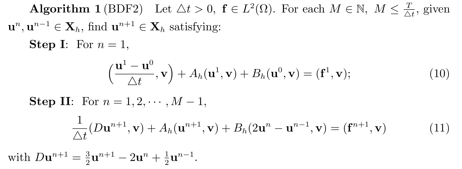
In this section, we propose two partitioned time stepping methods for (1)-(4). In both schemes, the coupling terms on the interface conditions are treated explicitly so that only two decoupled diffusion equations are solved at each time step. Therefore,subproblems can be implemented in parallel and the legacy code for each one can be utilized. Here, we denote the time step size by △t.

The first scheme, we discretize in time via a second-order BDF, whereas the interface term is treated via a second-order explicit Gear’s extrapolation formula. The BDF2 scheme states as below.

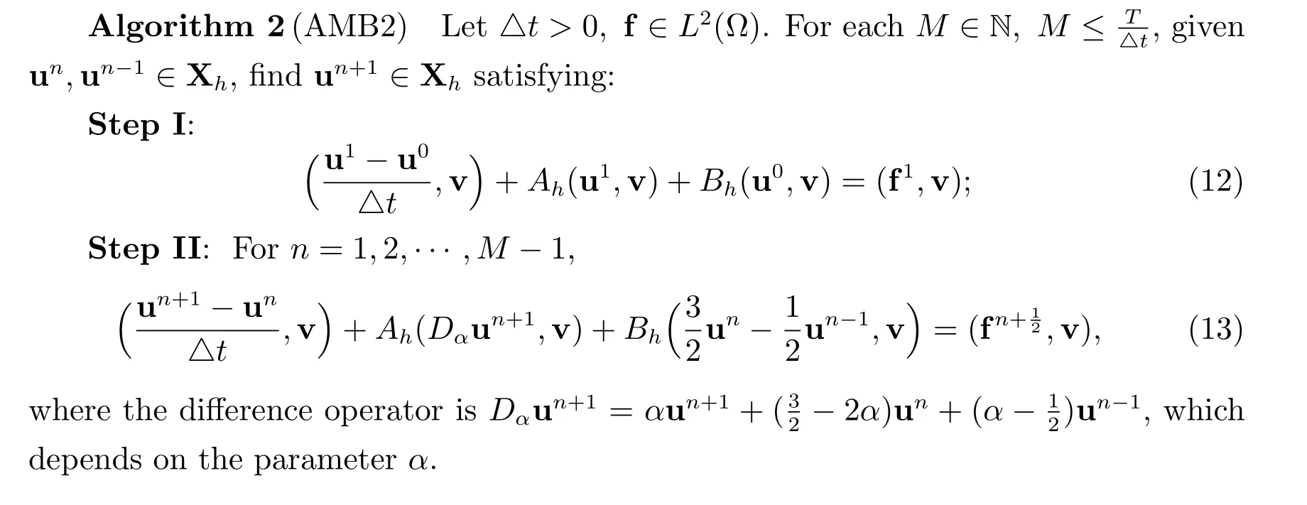
For the second scheme,we combine the second-order implicit Adams-Moulton treatment of symmetric terms and the second-order explicit Adams-Bashforth treatment of the interface term to propose the following second-order scheme.

4 Unconditional stabilities of the BDF2 and AMB2 schemes

To prove the unconditional stabilities of two second-order schemes proposed in section 3, we give some basic facts and notation first. The G-matrix associated with the classical second-order BDF is given by

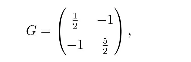
for any w ∈X2, define G-norm by |w|2G= 〈w,Gw〉. It is easy to verify that, for any vi∈X, i=0,1,2, we have

where w0= [v0,v1]Tand w1= [v1,v2]T. This G-norm is an equivalent norm on(L2(Ω))2in the sense that there exist Cl,Cu>0 such that

Besides, we also recall the following three basic inequalities:

Theorem 1(Unconditional stability of BDF2) Let T >0 be any fixed time,then Algorithm 1 is unconditionally by stable on (0,T].

Proof For Step I in Algorithm 1, we set v=u1in (10), it gives that

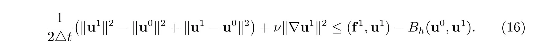
From Young’s and trace inequalities, we have

For Step II in Algorithm 1, by setting v=un+1in (11), we have

From (14), we have

where wn=[un+1,un]Tand δun+1=un+1−2un+un−1. Note that

Thus, by combining with (17), the unconditional stability of BDF2 is proved.

Next, to analyze the stability of AMB2 scheme, we introduce the following parameters

Substituting (30)-(32) into (29) yields

Define the energy

Then, by adding

to both sides, we have

5 Convergence of the BDF2 and AMB2 schemes

In this section,we study the convergence results of both BDF2 and AMB2 schemes.We assume that the mesh is regular and the parameter h denotes the grid size. We use continuous piecewise polynomial of degree l for both finite element spaces X1,hand X2,h.

Definition 1 For any u ∈X, define a projection Phu ∈Xhsatisfying

It is easy to verify that if u ∈(Hl+1(Ω1))d×(Hl+1(Ω2))d,we have the following property

To analyze the error estimate, we define the error at t=tnas

Theorem 3(Convergence of BDF2) Assume that the exact solution of the couping problem(1)-(4)is sufficient regular in the sense of u ∈H3(0,T;H1)∩H2(0,T;Hl+1),and the time-step restriction

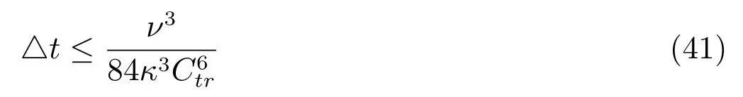
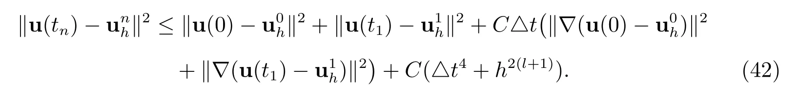
holds. Then, the solution of the BDF2 scheme satisfies the following error estimate

Proof By subtracting (11) from (9) at time tn, we derive the following error equation

From the definition of projection (38), (43) can be rewritten as

By setting vh=θn+1in (44), we have

Denote ϖn=[θn+1,θn]T, we discard the positive term Bh(θn+1,θn+1), it gives that

For the term Bh(δθn+1,θn+1),by using Cauchy-Schwarz inequality and trace inequality,we have

The terms on the RHS side of (47) can be bounded by using Young’s inequalities as

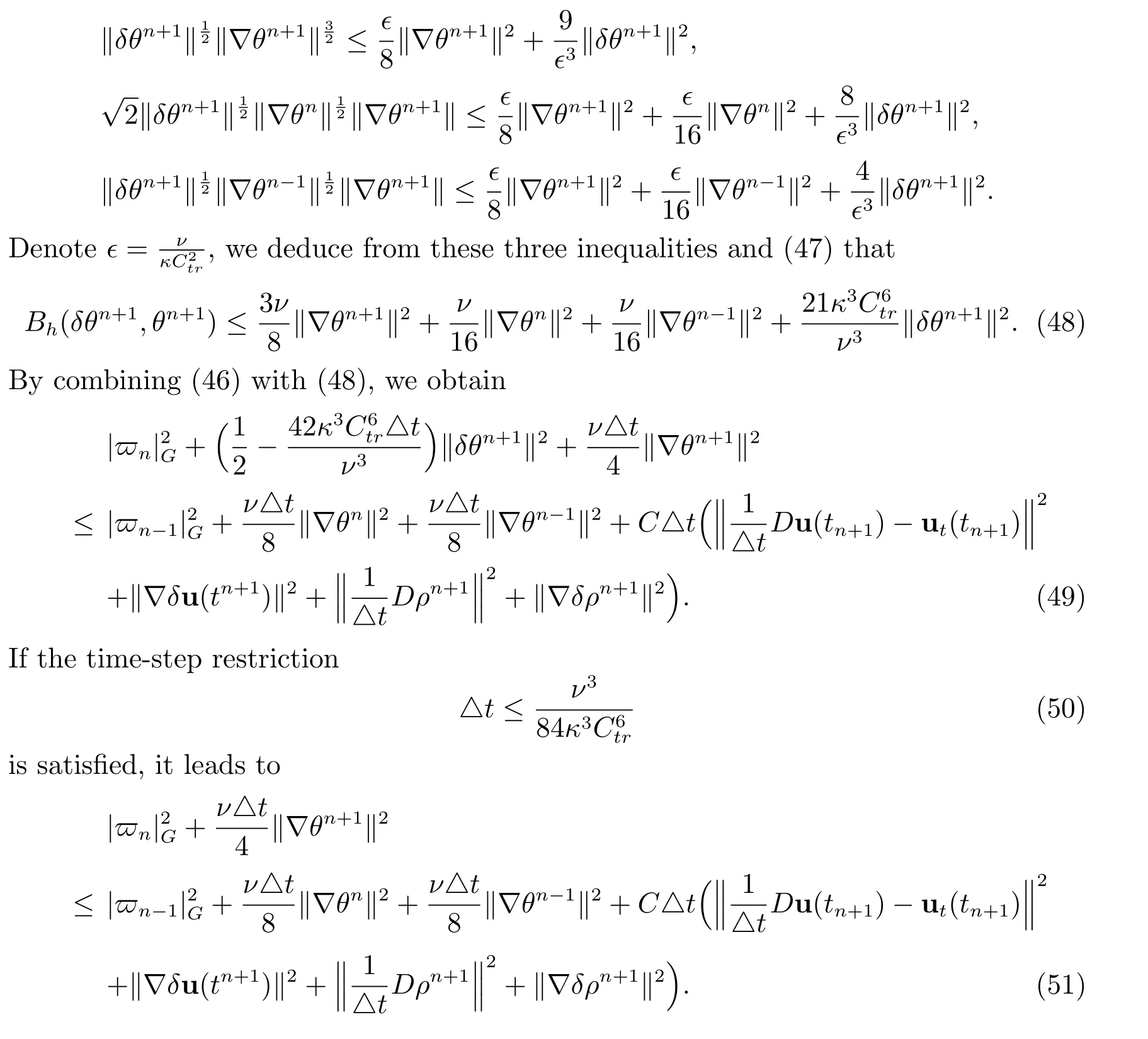
The desired error estimate follows from (58) and the interpolation error (39).

Theorem 4(Convergence of AMB2) Assume that the solution of the coupling problem (1)-(4) is sufficient regular in the sense of u ∈H3(0,T;H1)∩H1(0,T;Hl+1).Then the solution of AMB2 scheme satisfies the following error estimate

Proof By subtracting (13) from (9) at time tn+12, we derive the following error equation

It can be rewritten as

where we use the definition of projection

By setting vh=θn+1in (61), we derive

From Cauchy-Schwarz inequality, we have

and

For the interface term, there exists a constant C1, which is the same as that in (31)such that

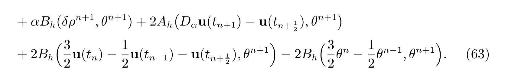
By combining these inequalities with (63), we obtain

and discard the second positive term on the LHS of (66), we have

For the terms on the RHS side of (68), we have

The same as (57), we have

From Taylor’s theorem with the integral form of the remainder, we have

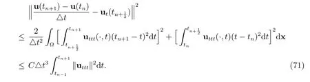
Similarly, we have

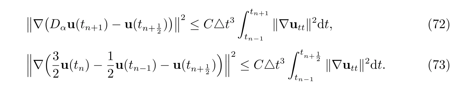
By combining (69)-(73) with (68) and discarding the positive terms on the LHS, we have

By recursion, we have

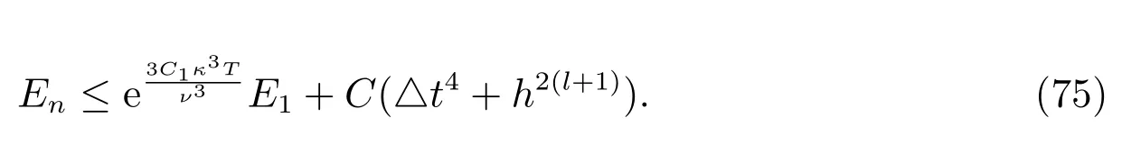
The desired error estimate follows from (75) and the interpolation error (39).

6 Numerical tests

In this section, we carry out the numerical experiments for BDF2 and AMB2 schemes. We focus on the convergent rates of both schemes. Assume that Ω1=[0,1]×[0,1] and Ω2=[0,1]×[−1,0], the interface I is the portion of the x−axis from 0 to 1. Then ˆn1= [0,−1]Tand ˆn2= [0,1]T. The forcing term f is chosen to ensure that the exact solutions are as follows[3]

u1(t,x,y)=ax(1 −x)(1 −y)e−t, u2(t,x,y)=ax(1 −x)(c1+c2y+c3y2)e−t,

with

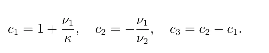
Computational results comparing the performance of two schemes are listed for two test problems:

Test problem 1: a=ν1=ν2=κ=1;

Test problem 2: a=4, ν1=5, ν2=10, κ=1/4.

For test problem 1, by setting △t=h with h=1/16, 1/32, 1/64 successively, we present the errors and convergent orders in Table 1 for both BDF2 and AMB2 with P1 finite element (here and later, we fix α = 0.8 for AMB2). The results illustrate the second-order in time accuracy for ‖un−unh‖. Besides, we notice that BDF2 has a significantly smaller error than AMB2. In Table 2, we set △t2= h3with h =1/8, 1/16, 1/32 and P2 finite element is chosen, the results illustrate the second-order in time accuracy and three-order in space accuracy for ‖un−unh‖. In this case, we can also find that BDF2 has a little better accuracy than AMB2. These results verify our theoretical results given in Theorem 3 and Theorem 4.

In the same way, in Table 3 and Table 4, we implement test problem 2 for both P1 and P2 finite element spaces,respectively. The expected convergence rates are obtained for BDF2 and AMB2 schemes.

Table 1 L2−error for BDF2 and AMB2 with P1, △t=h

Table 2 L2−errors for BDF2 and AMB2 with P2, △t2 =h3

Table 3 L2−errors for BDF2 and AMB2 with P1, △t=h

Table 4 L2−errors for BDF2 and AMB2 with P2, △t2 =h3

7 Conclusion

We proposed and investigated two second-order partitioned time stepping methods for a parabolic two domain problem. We have shown that our schemes are unconditionally stable and optimally convergent. The second-order partitioned methods for the fully nonlinear fluid-fluid problem is a subject of our future research.