Ji LI (李季)

College of Mathematics and Statistics, Chongqing Technology and Business University,Chongqing Key Laboratory of Social Economy and Applied Statisties, Chongqing 400067, China

E-mail :liji maths@email.ctbu.edu.cn

Carole ROSIER†

Universite du Littoral Cˆote d’Opale, UR 2597,LMPA, Laboratoire de Mathématiques Pures et Appliquées Joseph Liouville, F-62100 Calais, France,CNRS FR 2037, France

E-mail: rosier@univ-littoral.fr

Abstract This article is devoted to the identification, from observations or field measurements, of the hydraulic conductivity K for the saltwater intrusion problem in confined aquifers. The involved PDE model is a coupled system of nonlinear parabolic-elliptic equations completed by boundary and initial conditions. The main unknowns are the saltwater/freshwater interface depth and the freshwater hydraulic head. The inverse problem is formulated as an optimization problem where the cost function is a least square functional measuring the discrepancy between experimental data and those provided by the model.Considering the exact problem as a constraint for the optimization problem and introducing the Lagrangian associated with the cost function, we prove that the optimality system has at least one solution. Moreover, the first order necessary optimality conditions are established for this optimization problem.

Key words parameters identification;optimization problem;strongly coupled system;nonlinear parabolic equations; seawater intrusion

1 Introduction

In order to get an optimal exploitation of freshwater and then to control seawater intrusion in coastal aquifers,we need to develop efficient and accurate models to simulate the transport of saltwater front in coastal aquifer. Thus an essential step is to identify the parameters involved in the model.

In this article, we focus on the identification of physical parameters such as the hydraulic conductivity K and the porosity φ. The estimation of these parameters is based on observations or field measurements made on hydraulic heads and on the depth of the freshwater/saltwater interface. We note that concretely, there are only specific observations (in space and in time)corresponding to the number of monitoring wells.

We also emphasize that the parameters identification problematic was often addressed as part of the underground hydraulic(cf. [1–6]),but more rarely with regard to saltwater intrusion phenomena. The first studies done by Sun et Yeh (cf. [7]) develop the case of resolutions of inverse problem for coupled systems and provide, especially in the case of saltwater intrusion,the associated adjoint system corresponding to the steady system.

Moreover, we note that existing studies are mainly about numerical resolutions of these inverse problems. In particular, the study done in [8]has to be mentioned: the authors focus on the numerical resolutions of the hydraulic conductivity identification in the case of confined aquifers. The system of optimality is discretized by a finite element method; To solve the optimization problem, the authors used the C++ finite element library Rheolef and a C/C++program based on the advanced optimization package (TAO) that implements the BLMVM algorithm.

In [9], the authors proposed a theoretical study by proving the existence of an optimal control and they gave the necessary optimality conditions in the case of a steady saltwater/freshwater interface. But the seawater intrusion phenomenon is often transient and the study of sensitivity proposed in [10]shows that the form of freshwater/saltwater interface depends mainly on the hydraulic conductivity. The other parameters such as especially porosity,have an impact on the time taken to reach the steady state, which is, why the unsteady model has to be considered to identify simultaneously both parameters.

The current article is a generalization of [9]to the unsteady case. The inverse problem then reduces in an optimization problem, where the cost function is a least square functional measuring the discrepancy between experimental data and those given by the model. Clearly,the time dependance of the variables is one of the difficulties of this study. Then, taking the exact problem as a constraint of the optimization problem, we introduce the Lagrangian associated with the cost function. In the field considered here, the effects due to porosity variations are negligible compared to those due to the density contrasts. We thus assume that porosity is constant in the aquifer and we only focus on the hydraulic conductivity identification.

Before detailing the mathematical analysis of this optimization problem, let us describe briefly the derivation of the model. We refer to the textbooks [11–13]for general informations about seawater intrusion problems. The basis of the modeling is the mass conservation law for each species (fresh and salt water)combined with the classical Darcy law for porous media. In the present work we have essentially chosen to adopt the simplicity of a sharp interface approach.Indeed, observations show that, near the shoreline, fresh and salty underground water tend to separate into two distinct layers. It was the motivation for the derivation of seawater intrusion models dealing with salt and freshwater as immiscible fluids. Nevertheless the explicit tracking of the interfaces remains unworkable to implement without further assumptions. An additional assumption, the so-called Dupuit approximation, consists in considering the hydraulic head as a constant along each vertical direction. It allows to assume the existence of a smooth sharp interface. Classical sharp interface models are then obtained by vertical integration based on the assumption that no mass transfer occurs between the fresh and the salty area (see e.g.[12]and even the Ghyben–Herzberg static approximation). This class of models allows direct tracking of the salt front. Nevertheless the conservative form of the equations is perturbed by the upscaling procedure. In particular the maximum principle does not apply. Following[14], we can mix the latter abrupt interface approach with a phase field approach (here an Allen–Cahn type model in fluid-fluid context see e.g. [15–17]) to re-include the existence of a diffuse interface between fresh and saltwater where mass exchanges occur. We thus combine the advantage of respecting the physics of the problem and that of the computational efficiency.Theoretically speaking, an advantage resulting from the addition of diffuse area compared to the sharp interface approximation is that the system now has a parabolic structure. So it is not necessary to introduce viscous terms in a preliminary fixed point to deal with degeneracy as in the case of sharp interface approach (cf. [14]). The second advantage is that we can prove the uniqueness of the solution by establishing a regularity result on the gradient of the solution.More precisely we generalize to the quasilinear case,the regularity result given by Meyers([18])in the elliptic case and extended to the parabolic case by Bensoussan,Lions and Papanicolaou,for any elliptic operatorThe results assume that the operator A satisfies a uniform ellipticity assumption and that its coefficients are functions of L∞(Ω).The hypothesis on A ensure the existence of an exponent r(A) > 2 such that the gradient of the solution of the elliptic equation(resp. of the parabolic equation)belongs to the space Lr(Ω)(resp. Lr(ΩT)). This additional regularity combined with the Gagliardo-Nirenberg inequality can handle the nonlinearity of the system in the proof of the uniqueness. For these reasons,we limit ourselves in this paper to the case of diffuse interface approach.

The first difficulty of the work consists in choosing appropriately the set of all eligible parameters. Taking this set in space L∞(Ω)ensures the existence and uniqueness of the solution of the initial problem but does not provide the existence of the optimal control problem. Also taking this set in H1(Ω) is a too restrictive hypothesis that must be weakened. Therefore we introduce the set of admissible parameters defined as a subset of the space BV(Ω), the space of bounded variation functions, in order to recover discontinuous coefficients. On the other hand, the total variation of the control variables is assumed to be uniformly bounded, so as to ensure the compactness result useful to prove the existence of an optimal control. Then, we establish that the associated adjoint state system admits a unique solution. This retrograde problem consists in a strongly coupled system of linear elliptic-parabolic equations, the main difficulty is related to the presence of scalar products between the gradients of the exact solution and those of the unknowns. The L4-regularity result obtained for the direct problem allows to deal with these terms. We thus use a Schauder fixed point theorem to prove the existence result. The second difficulty comes from the operator associating the state variables with the hydraulic conductivity. We have to establish that it is continuous and differentiable on a suitable functional spaces. At this point, the main difficulty consists in defining the suitable function spaces so that the requirements of the implicit function theorem can be satisfied. Again,the Lσregularity of the exact solution (for σ >4) is fundamental in order to prove the continuity and differentiability of the previous operator. Finally,the first order necessary optimality conditions are established.

This article is organized as follows: In Section 2.1 we present the seawater intrusion problem.We also recall the essential properties of the space of functions with bounded variations and we state the main Theorems of the paper. In Section 3 all mathematical notations are given.Furthermore the global in time existence and uniqueness results are stated in the confined case with sharp-diffuse interface approach. The Section 4 contains the proofs of main results of the paper. We first prove the existence of the optimal control. Considering the system as a constraint for the optimization problem, we introduce the Lagrangian function associated with the cost function. We establish the existence and uniqueness results for the adjoint problem. We prove that the operator associating with the hydraulic conductivity the corresponding solution of the exact problem, is continuous and differentiable. The main point consists in finding the well adapted function spaces so that the implicit function theorem is applicable. Finally, we state the first order necessary optimality conditions for the optimization problem.

2 Problem Statement and Main Results

2.1 Problem statement

We consider an open bounded domain Ω of R2describing the projection of the aquifer on the horizontal plane. The boundary of Ω, assumed C1, is denoted by Γ. The time interval of interest is(0,T),T being any nonnegative real number,and we set Ωτ=(0,τ)×Ω, ∀τ ∈ (0,T).The confined aquifer is assumed to be bounded by two layers,the lower surface corresponds to z =h2and the upper surface to z =h1. Quantity h2−h1represents the total thickness of the aquifer (cf. Figure 1). We assume that depths h1, h2are constant, such that h2>δ1>0 and without lost of generality we can set h1=0.

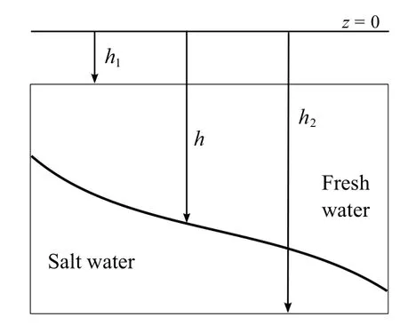
Figure 1 Schematization of an aquifer

In the case of confined aquifer, the well adapted unknowns are the interface depth h and the freshwater hydraulic head f. The nonnegative function K represents the hydraulic conductivity (which is assumed to be a scalar), φ denotes the porosity, δ the thickness of the diffuse saltwater/freshwater interface(δ =0 corresponds to the classical sharp interface approach)and the parameter α characterizes the densities contrast:

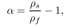
where the characteristics ρsand ρfare respectively the densities of saltwater and freshwater.

Thus, the model reads (see [8, 20]):

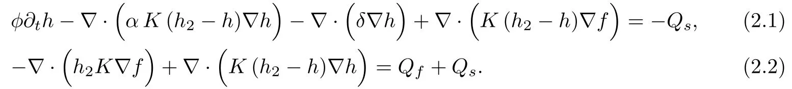
In the previous system,the second equation models the conservation of total mass of water,while the first is modeling the mass conservation of saltwater. This is a 2D model, the third dimension being preserved by the upscaling process via the depth information h.

The system (2.1)–(2.2) is completed by the following boundary and initial conditions:

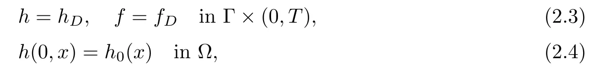
with the compatibility condition

Let us now introduce some elements for the functional setting used in the present paper. For the sake of brevity we shall write H1(Ω)=W1,2(Ω) and

The embeddings V ⊂ H =H′⊂ V′are dense and compact. For any T >0,let W(0,T)denote the space

The inverse problem is formulated by an optimization problem whose cost function measures the squared difference between the depths of experimental interfaces depths and those given by the model. We introduce the following control problem:

where (f(K),h(K)) denotes the solution of the variational problem (2.1)–(2.2) completed by the boundary and initial conditions (2.3)–(2.4). The functions (fobs,hobs) correspond to the observed hydraulic head and depth of the freshwater/salt water interface.

We thus propose to work on the set of admissible parameters:

where K−, K+and c are nonnegative real constants. This choice of set allows to recover discontinuous coefficients for the hydraulic conductivity.

We denote by BV(Ω) the space of functions in L1(Ω) with bounded variation on Ω, which is a Banach space for the norm

Definition 2.1Let g be a function of L1(Ω); we call total variation of g on Ω the real

g is a function with bounded variation if TV(g)<∞.

We remind that Uadmis a compact subset of Lr(Ω) for all r ∈ [1,+∞[, we refer the reader to [21]for more details about that.

2.2 Main results

Existence of optimal control

Since the total variation of the control variables is assumed to be uniformly delimited, this ensures a compactness result for the set Uadmin L2(Ω). This property combined with the uniqueness of the exact solution leads to the existence of a solution for the control problem.

Theorem 2.2There exists at least one optimal control for the problem (O).

Existence and uniqueness results for the adjoint problem

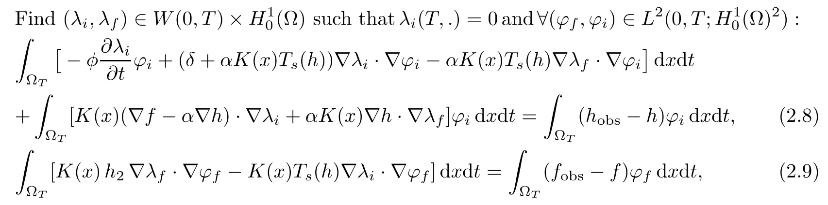
By considering the exact problem as a constraint for the optimization problem and introducing the Lagrangian associated with the cost function, we define the associated adjoint state problem given by the following retrograde system:

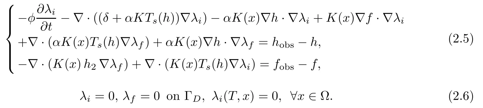
Then we prove the well-posedness of system (2.5)–(2.6):

Theorem 2.3Assuming that the hydraulic conductivity satisfies

Let (f,h) be the solution of (2.1)–(2.4) associated with the hydraulic conductivity K ∈ Uadm,the adjoint problem defined by

has a unique solution.

Optimality conditions

In order to state the first order necessary optimality conditions for the problem(O),we first aim to check that the operator, denoted by Q, associating the solution (f(K), h(K)) of (2.1)–(2.4) with the hydraulic conductivity K, is continuous and differentiable on suitable function spaces. The main point consists in finding the well adapted function spaces so that the implicit function theorem is applicable. It can be possible if the gradient of the solution of the exact problem is sufficiently regular, namely iffor s > 2. We thus introduce the following spaces

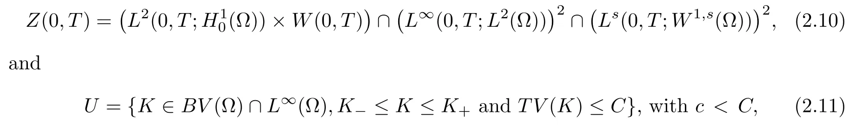
where the constant c is the constant definingIn these spaces,the following Theorem holds true

Theorem 2.4Assume the condition (2.7) is satisfied. The mapping Q is continuous and differentiable from Uadmto Z(0,T).

By collecting all the previous results, we directly verify that the minimum required, K∗,satisfies the optimality system and thus establish the following result

Theorem 2.5Assume the condition (2.7) is satisfied. Let K∗be a solution of problem(O), there exists a coupleand a couple λ∗=satisfying the optimality system determined by the direct problem (2.1)–(2.4), the adjoint problem (2.5)–(2.6) and, for all K ∈ Uadm

with the gradient of the cost function given by, ∀δK∈ Uadm

3 Global in Time Existence and Uniqueness Results

We introduce function Tsdefined by

The function Tsis extended continuously and by constants outside (δ1,h2). It represents the thickness of the saltwater zone in the reservoir, the previous extension of Tsfor h ≤ δ1enables to ensure a thickness of freshwater zone inside the aquifer always greater than δ1. Let us now detail the mathematical assumptions. We begin with the characteristics of the porous structure. We assume the existence of two positive real numbers K−and K+such that the hydraulic conductivity K is nonnegative and uniformly bounded, namely

We suppose that porosity φ is constant in the aquifer. Indeed, in the field envisaged here, the effects due to variations in φ are negligible compared with those due to density contrasts. From a mathematical point of view, these assumptions do not change the complexity of the analysis but rather avoid cumbersome computations. We remind that the parameter δ represents the thickness of the diffuse saltwater/freshwater interface, it is of order of 1 m.

Source terms Qfand Qsare given functions of L2(0,T;H) and we assume that Qf≥0 and Qs≤0.

Functions hDand fDbelong to the spaceH1(Ω)) while the function h0is in H1(Ω) Finally, we assume that the boundary and initial data satisfy conditions on the hierarchy of interfaces depths:

We first recall the global existence result established in [20]:

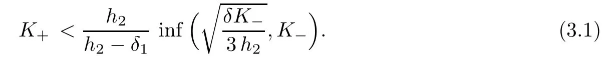
Theorem 3.1Assume a low spatial heterogeneity for the hydraulic conductivity tensor:

Then for any T >0, problem (2.1)–(2.4) admits a weak solution (h,f) satisfying

Furthermore the following maximum principle holds true:

Remark 3.2We emphasize that the depth h is naturally bounded by two quantities characterizing the aquifer as shown by the maximum principle established in Theorem 3.1.This result is specific to confined aquifers, it is no longer valid in the case of free aquifers, for which one can find oneself in situations of overflow of the aquifer.

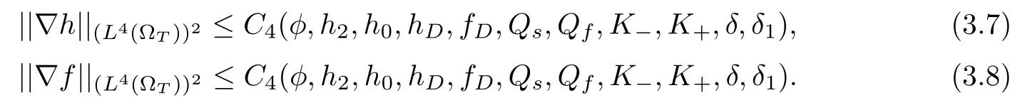
The following uniqueness result is a consequence of a Lr(0,T;W1,r(Ω)), r > 2, regularity result proved for the solution of (2.1)–(2.2). This regularity is a generalization of the Meyers regularity results [18]given in elliptic case and extended in parabolic case in [19]. We first introduce some useful notations.

• Elliptic case

We recall the following result (see Lions and Magenes [22]):

We set G = (−∆)−1andWe notice that g(2) = 1. We thus introduce, for any real number c>0

the positivity of c ensuring ν < µ. We consider r,r >2 such that k(r):=g(r)(1 − µ + ν)<1.Letting c →0, the condition k(r)<1 yields

The condition(3.3)implies a low spatial heterogeneity for the hydraulic conductivity,so as the assumption (3.1).

• Parabolic case

Again we introduce, for any real number ˆc>0

We thus can state the following Theorem (cf.[20]):

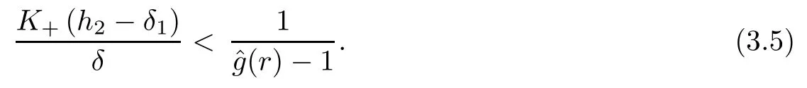
Theorem 3.3Letsatisfying (3.1), (3.3) and (3.5) for r = 4.Furthermore we assume that there exists γ,0< γ <1,such that the physical parameters satisfy

If h0∈ W1,4(Ω), (hD,fD) ∈ L4(0,T;W1,4(Ω))2and (Qs,Qf) ∈ L4(ΩT)2, then the solution of the system (2.1)–(2.4) is unique inMoreover, we have

Remark 3.4Assumption(3.1)(so as(3.3)and(3.5))makes only sense when considering low values for K. For the present application, this point is not restrictive since the soil permeability typically ranges from 10−8to 10−3m·s−1. A priori, assumption (3.6) is stronger than(3.5) except if δ1, the thickness of freshwater zone inside the aquifer, is sufficiently large.

By now, we suppose that the hydraulic conductivity K satisfies (3.1), (3.3), (3.5)and(3.6)in order to guarantee the existence and the uniqueness of the solution of (2.1)–(2.4).

4 Identification of Hydraulic Conductivity

In this section, we prove the results that constitute the four steps to solve this inverse problem. We first of all show that the control problem admits a solution. Then, by considering the exact problem as a constraint for the optimization problem and introducing the Lagrangian associated with the cost function, the solution is characterized by the optimality system it must satisfy.

4.1 Proof of Theorem 2.2

The two keys to this proof are on the one hand the compactness of Uadmin L2(Ω) and on the other hand the uniqueness of the solution of the exact problem.

Let (Kn)n∈N⊂ Uadmbe a minimizing sequence (which exists due to the boundedness of the functional J in R) such that

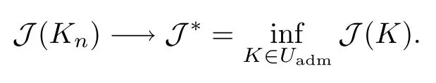
Since Uadmis a compact subset of L2(Ω), we deduce there exists a subsequence, still denoted Kn, and a function K∗∈Uadmsuch that

In an other hand, the solution (fn,hn)=(f(Kn),h(Kn)) of the variational problem, satisfies:

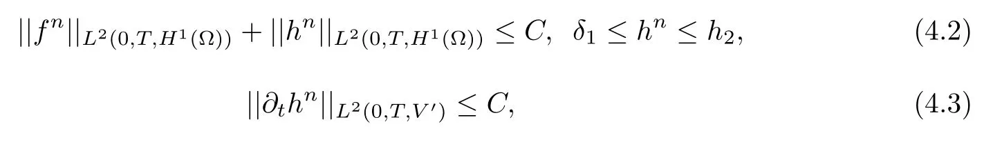
where C is a constant independent on n.

Then (hn)nis uniformly bounded in W(0,T), we deduce from Aubin compactness result that the sequence (hn−hD)nis sequentially compact in L2(0,T,H). Furthermore (fn)nis sequentially weakly compact in L2(0,T;H1(Ω)).

We can therefore extract a subsequence, not relabeled for convenience, (fn,hn− hD)n∈L2(0,T;H1(Ω))×W(0,T)and there exits(f∗,h∗−hD)∈ L2(0,T;H1(Ω))×W(0,T)such that:

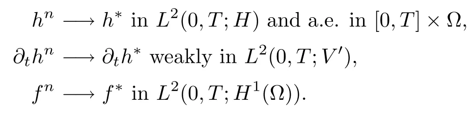
This allows to pass to the limit in the variational formulation corresponding to exact problem(2.1)–(2.4).

From the uniqueness of the solution, it follows that:

This ends the proof.

4.2 Definition of the Lagrangian L

The minimum of the cost function J has to be determined, the state system being the unsteady problem (2.1)–(2.4). We consider this system as a constraint for the optimization problem, where the Lagrangian L is defined as follows:

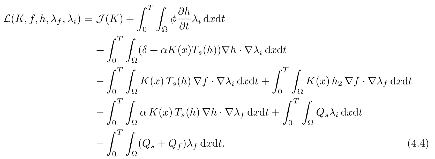
The solution thus corresponds to a saddle point of L considered as function of independent variables h, f,λi,λfand K with λiand λfthe Lagrange multipliers. The minimum, K∗,satisfies the following optimality system:

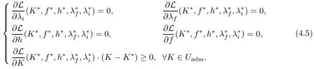
where(h∗,f∗)is the unique solution of(2.1)–(2.4)for K =K∗andthe unique solution of the adjoint system (2.5)–(2.6) for K =K∗.

4.3 Adjoint problem - Proof of Theorem 2.3

Since the system(2.5)–(2.6)is retrograde,we firstly set t′=T −t,the system thus becomes:

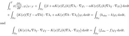
The initial condition is now written as λi(0,x)=0,∀x ∈ Ω.

This is a coupled system of elliptic-parabolic linear equations. From now on, we omit the prime in t′.

To prove the existence of the solution of (4.6)–(4.6), we will proceed as for the proof of global existence in the confined case with diffuse interfaces (cf. [20]). We emphasize that the only difficulty, in this case, is the presence of linear terms K(∇f −α∇h)·∇λiand K∇h·∇λfwhich simultaneously involve the gradients of solutions of the exact problem and the adjoint problem. The result of regularity (3.7)–(3.8) established in Theorem 3.3 makes it possible to overcome this technical difficulty. In addition, since the system (2.5)–(2.6) is strongly coupled,a fixed point strategy is used to reduce it to the classic theory of linear problems.

Global in time existence

For the strategy of fixed point, we introduce the application F :

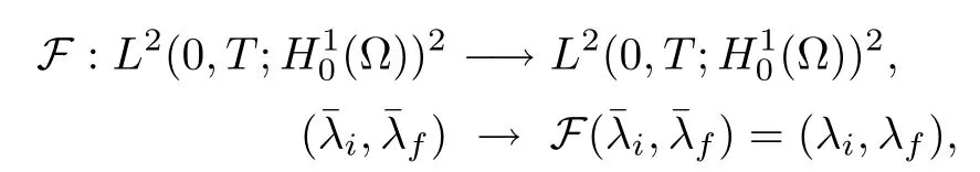
We know from the classical theory of linear parabolic equations that the previous variational system has a unique solution. We first have to prove the continuity of F,that is the continuities of F1and F2.

Sequential continuity of F1in L2(0,T;H) when F is restricted to any bounded subset of W(0,T)× L2(0,T;H1(Ω)).

We thus have

Moreover, thanks to Cauchy-Schwarz,Young and Gagliardo-Nirenberg inequalities, we get∀ǫ>0

By gathering together all these inequalities, we obtain

Choosing ǫ>0 such that δ − ǫ>0 andwe established that there are two reals AM(h,hobs, f,K,α,C4,δ,φ,h2,T) and BM(h,hobs, f,K,α,C4,δ,φ,h2,T) depending only on the data such that

The sequence (λi,n)nthus is uniformly bounded inWe set CM=max(AM,BM).

We now establish that (∂tλi,n)nis bounded inso we have

As the principle of the calculations is the same as for the above inequalities, we only provide key estimates:

We can conclude that

where DMdepends only on the data and on M.

Thus (λi,n)nis uniformly bounded in the space

Using the Aubin Lemma, we can extract a sequence (λi,n)n, not relabeled for simplicity,that strongly converges in L2(ΩT) and weakly into a limit λl.

Thanks to the strong convergence of (λi,n)nin L2(ΩT) (and then the convergence a.e. inΩT), we can check that λlis a solution of (4.6). The solution of (4.6) being unique, we have λi= λland that the whole sequence λi,n→ λiweakly in W(0,T) and strongly in L2(0,T;H).The sequential continuity of F1in L2(0,T;H) is established.

Continuity of F2in L2(0,T;H) when F is restricted to any bounded subset of W(0,T)×L2(0,T;H1(Ω)):

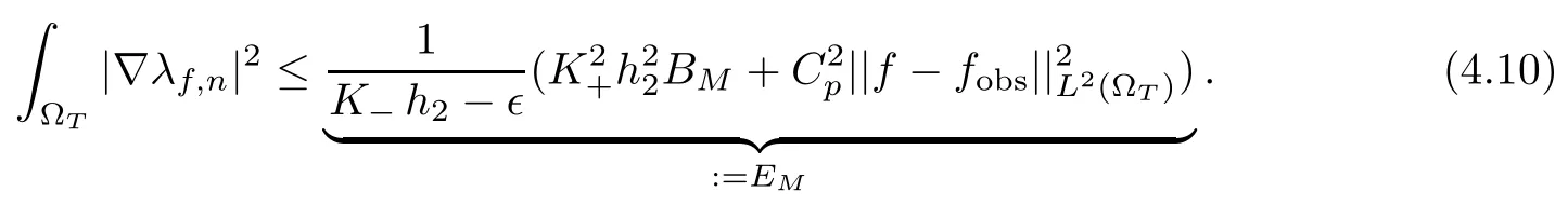
Similarly, we study the sequential continuity of F2by settingand showing first that λf,n→λfin L2(0,T;H1(Ω)) weakly. Key estimates are obtained using the same type of arguments as those used to prove the sequential continuity of F1. The details are therefore omitted. We only point out that we can use the estimate (4.15)previously derived for λi,nto obtain the following estimates for λf,n, for ǫ>0:

where Cpis the constant in Poincaré’s inequality.

Choosing ǫ such that K−h2− ǫ>0, we get

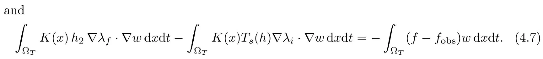
For proving the sequential compactness of λf,nin L2(0,T;H),we need some further work since we can not use a Aubin’s compactness criterium in the elliptic context characterizing λf,n.We actually get a stronger result: we claim and prove that λf,nconverges in L2(0,T;H1(Ω)).Indeed, we recall that the variational formulations defining respectively λf,nand λfare, for any w ∈L2(0,T;V),

The system (4.11)–(4.12) can be written as follows

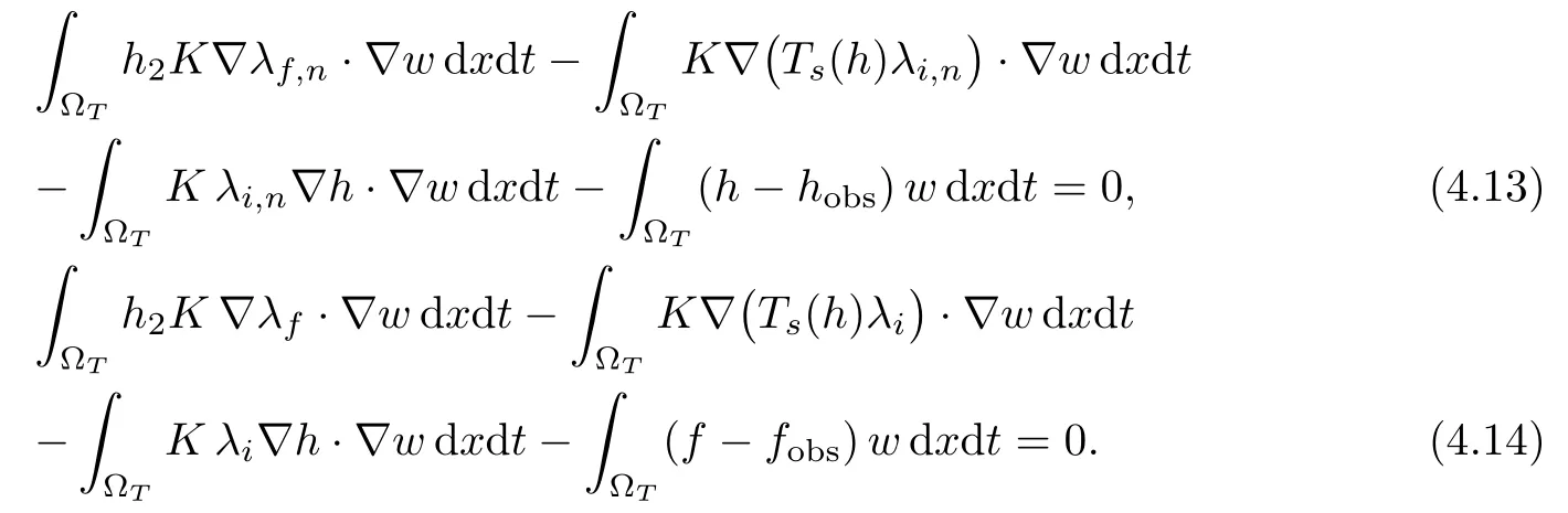
Choosing w = h2λf,n− Ts(h)λi,nin (4.13), we let n → ∞. The already known convergence results let us pass to the limit in

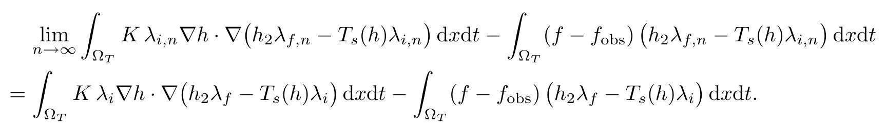
Moreover using (4.14) for the test function w =h2λf− Ts(h)λi, we conclude that

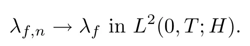
if Fn=h2λf,n−Ts(h)λi,nand F =h2λf−Ts(h)λi. Since Kξ·ξ ≥ K−|ξ|2for any ξ ∈ R2with K−>0, the latter result and the Poincaré inequality let us ensure that Fn→ F in L2(0,T;V).Since h2>0, it follows in particular that

Existence of C ⊂ W(0,T)× L2(0,T;(H1(Ω)) such that F(C)⊂ C.

We aim now to prove that there exists a nonempty bounded closed convex set of W(0,T)×L2(0,T;H1(Ω)), denoted by C, such that F(C)⊂ C.

We notice that this result will imply that there exists a real number> 0, depending only on the initial data, such that for∈W, we have

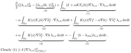
Taking λi∈ L2(0,T;V) (resp. α λf∈ L2(0,T;V)) in (4.6) (resp. in (4.7)) and adding the two resulting equations lead to:

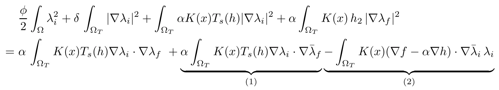
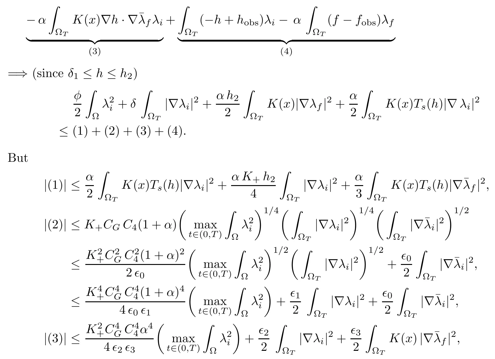
finally, using Poincaré’s inequality (with constant CP) yields

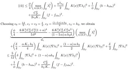
We assume that the coefficient φ is big enough in order to ensure the nonnegativity of Θ1,namely

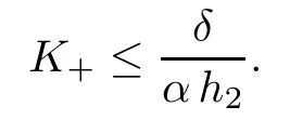
and that the hydraulic conductivity satisfies (2.7) given in Theorem 2.3:

We then choose the constant M >0 such that

hence we can conclude that

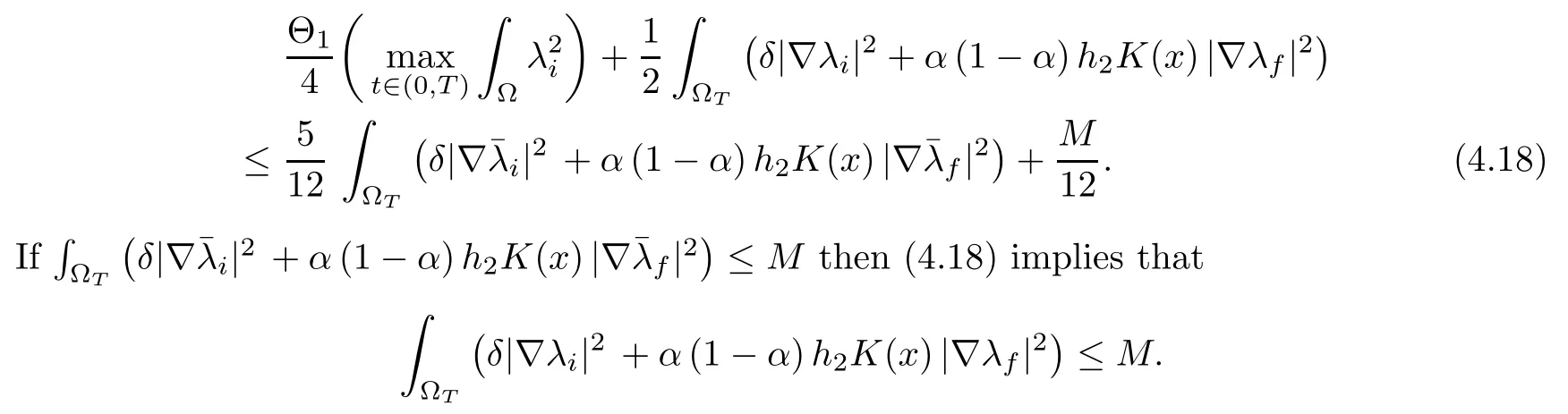
Setting C the nonempty bounded closed convex set of W(0,T)×W(0,T) defined by:

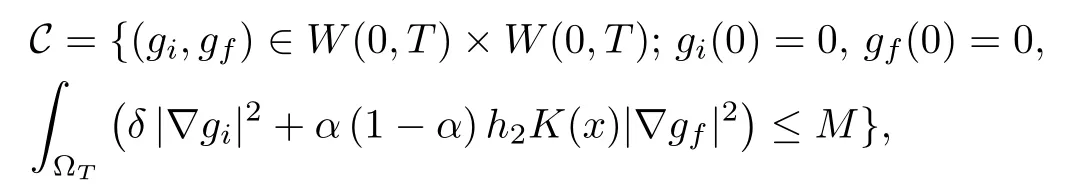
we established that F(C)⊂C. Then C is a nonempty closed convex bounded set of L2(0,T;H)2,defined such that F(C) ⊂ C. Since C is also a bounded set in W(0,T))× L2(0,T;H1(Ω)), we also proved that F restricted to C is sequentially continuous in (L2(0,T;H))2. For the fixed point strategy, it remains to show the compactness of F(C). Since we work in metric spaces,proving its sequential compactness is sufficient. The compactness of F1(C) is straightforward due to the Aubin’s theorem. Let us further detail the proof for F2(C). Let{λf,n}be a sequence in F2(C). It is associated with a sequencein C. The Aubin’s compactness theorem let us ensure that there exists a subsequence, not renamed for convenience, andsuch thatin L2(0,T;H) and almost everywhere in ΩT. Thus we can follow the lines beginning just after (4.10) for proving that λf,n→ λfin L2(0,T;H). The sequential compactness of F2(C) in L2(0,T;H) is proved. The Schauder theorem allows us to conclude that there is a couple (λi,λf) ∈ C such that F(λi,λf) = (λi,λf). This fixed point is a weak solution of the problem (4.6)–(4.6).

Uniqueness of the solution of the adjoint problem:

Let(λi,λf)∈W(0,T)2and∈W(0,T)2be two solutions of (2.9). We set u=Clearly, since the system is linear, (u,v) satisfies (2.9) but the right member of (2.9) is equal to zero.

The previous estimates lead to the following inequality

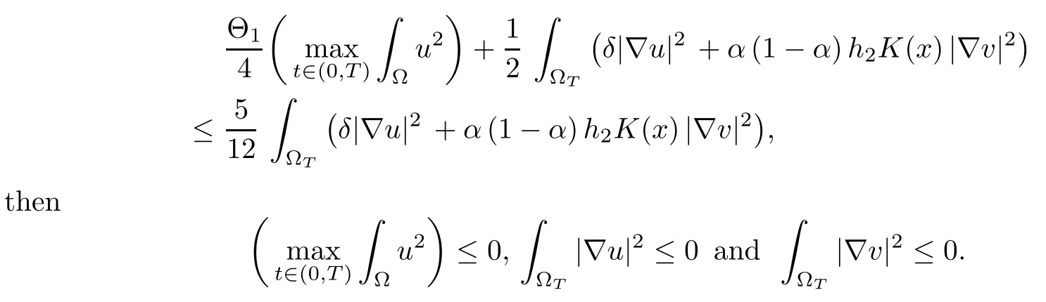
The condition (4.16) may look very restrictive. However, we can again pick the coefficient φ arbitrary large(for it corresponds to a time scaling),so that the conditions(4.16)can indeed be satisfied. Setting

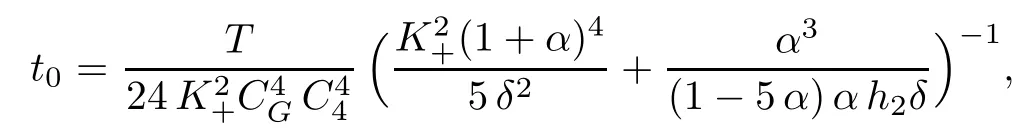
we proved the existence and the uniqueness for the short time t ∈[0,t0]. Taking t = t0as new initial data, the existence and uniqueness is obtained for all t0≤ t ≤ 2 t0. Using this observation inductively, we derive the result on the whole range of study [0,T]. This ends the proof of Theorem 2.3.

Remark 4.1The condition (2.7) is of the same type as the one involved in the theorem 3.3 giving the result of uniqueness. Since α =0.0125, δ =O(1) and h2=O(10), the condition(2.7) is not so restrictive.

4.4 Optimality conditions

To characterize a solution to the optimization problem(O),the gradient of the cost function is calculated using the Lagragian defined by(4.4). An essential step is to prove that the operator associating the solution (f(K), h(K)) of (2.1)–(2.4) with the hydraulic conductivity K, is continuous and differentiable. The main point is to find the appropriate function spaces for the implicit function theorem to be applicable. The regularity results established for(f(K), h(K))in Theorem 3.1 and the following Proposition 4.2 allow to conclude.

4.4.1 Proof of Theorem 2.4

The first results regarding these additional regularity is given in the following proposition

Proposition 4.2Let (f(K), h(K)) the solution of (2.1)–(2.4) associated with the hydraulic conductivity K ∈ Uadm. For all (Fi,Ff)∈ L2(0,T;H−1(Ω))2, the following problem

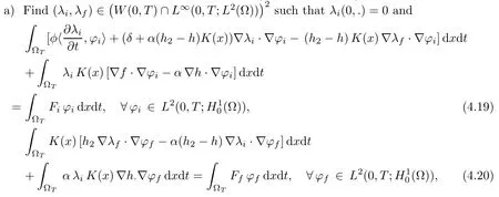
has one and only one solution.

ProofThe proof of a) of Proposition (4.2) is quite similar to the proof of Theorem 2.3,for this reason, we omit it here.

Regarding point b), we use again the Meyers regularity result by remarking that, sinceandwe can find s ∈]2, σ[ s.t. div(λi∇h) belongs to Ls(0,T;W−1,s(Ω)) (and the same for terms with f).Indeed∀pwith σ >4,then

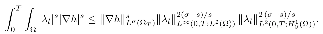
We directly deal with the other terms of (4.20) since functions h belongs to L∞(ΩT).

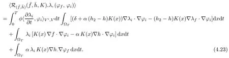
To prove the differentiability of the operator Q, we introduce an application R, defined as a function ofThe equality (4.24) below giving R allows to implicitly define Q. Applying the implicit function theorem to R, we thus deduce the differentiability of Q.

So, we consider the mapping R such that

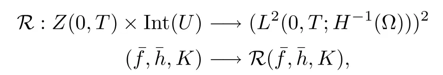
where Z(0,T)(resp. U)is defined by(2.10)(resp. by(2.11))and=(f −fD,h−hD). We note that Uadm⊂ Int(U), ‘Int’ denoting the interior of U for the topology of(cf. [9]).

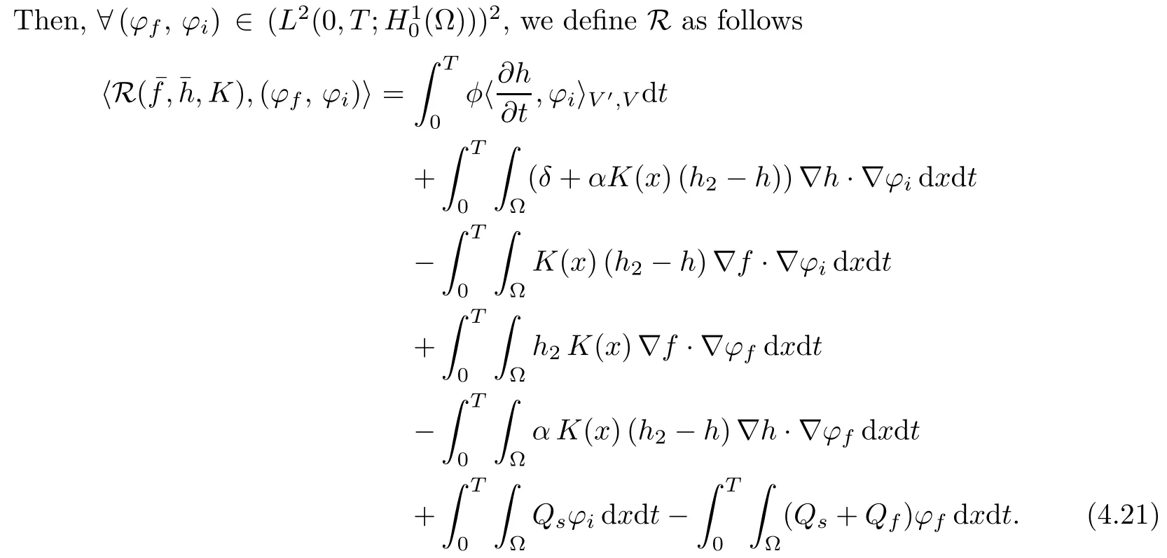
First of all,we notice that R(¯f(K),¯h(K),K)=0 since(f(K),h(K))is the solution of the state problem corresponding to the hydraulic conductivity K.

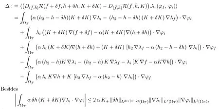
We now aim to prove that R is continuous and differentiable from Z(0,T)×Int(U) to(L2(0,T;H−1(Ω)))2. Since function h belongs to L∞(ΩT), the continuity of R is clear. Analogously, R is continuously differentiable with respect to K on Z(0,T)× Int(U) and for all L ∈Int(U)

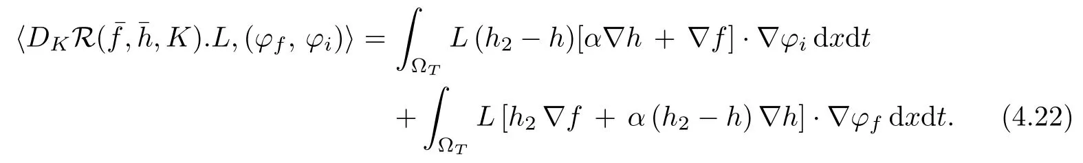
So, a direct calculation gives

We thus deduce the differentiability of R with respect toon Z(0,T)×Int(U) at the pointis solution of (2.1)–(2.2)). Furthermore,the partial differentialis defined by (4.23).

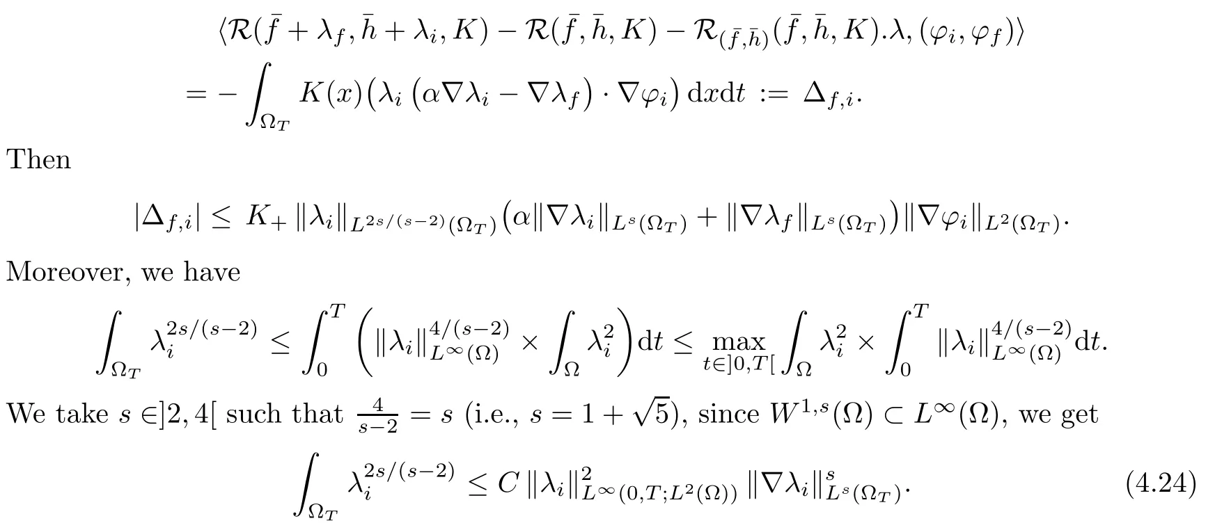
we conclude thanks to (4.24). Making similar estimates with the other terms of ∆, we deduce the continuity ofin a neighborhood of (f(K),h(K),K) in Z(0,T)×Int(U).

Moreover, Proposition 4.2 ensures thatis an isomorphism from Z(0,T)to(L2(0,T;H−1(Ω)))2, ∀K ∈ Uadm. The requirements of implicit function theorem are satisfied. This ends the proof of Theorem 2.4.

4.4.2 Proof of Theorem 2.5

The last step in the identification process is to demonstrate that the required minimum,K∗, satisfies optimality system (4.5).

Thanks to Theorem 2.4, the application K −→ Q(K) = (f(K), h(K)) implicitly defined by the direct problem (2.1)–(2.4), is differentiable.

So the application K −→ J(K)) = L(K,f(K),h(K),λi,λf) is differentiable with respect to (K,f,h) and

where the Lagrangian L is defined by (4.4)andFurthermore,every minimum of J on Uadmverifies (2.12).

Besides, the gradient of the cost function is given by, ∀δK∈ Uadm

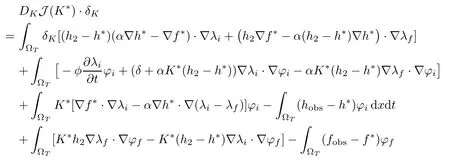
with h∗= h(K∗), f∗= f(K∗). We deduce from Theorem 2.3, that the adjoint problem has a unique solutionthen takingin(4.25) leads to (2.12), which ends the proof of Theorem 2.5.