Shulan HU (胡淑兰)

School of Statistics and Mathematics, Zhongnan University of Economics and Law,Wuhan 430073, China

E-mail :hu shulan@zuel.edu.cn

Ruinan LI (李瑞囡)

School of Statistics and Information, Shanghai University of International Business and Economics,Shanghai 201620, China

E-mail :ruinanli@amss.ac.cn

Xinyu WANG (王新宇)†

School of Mathematics and Statistics, Huazhong University of Science and Technology,Wuhan 430074, China

E-mail :wang xin yu@hust.edu.cn

Abstract In this paper we prove a central limit theorem and a moderate deviation principle for a class of semilinear stochastic partial differential equations, which contain the stochastic Burgers’ equation and the stochastic reaction-diffusion equation. The weak convergence method plays an important role.

Key words stochastic Burgers’ equation; stochastic reaction-diffusion equation; large deviations; moderate deviations

1 Introduction

For any ε > 0, consider the semilinear stochastic partial differential equation (SPDE for short)

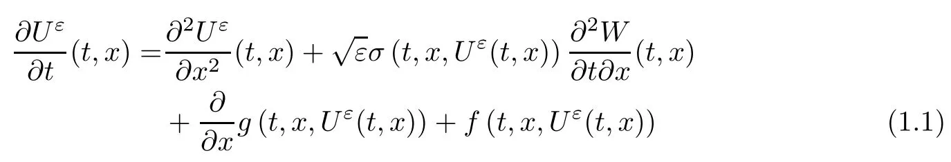
for all (t,x) ∈ [0,T]× [0,1], with Dirichlet boundary conditions (Uε(t,0) = Uε(t,1) = 0) and initial condition Uε(0,x) = η(x) ∈ Lp([0,1]),p ≥ 2; W denotes the Brownian sheet defined on a probability space (Ω,F,{Ft}t≥0,P); the coefficients f =f(t,x,r),g =g(t,x,r),σ = σ(t,x,r)are Borel functions of (t,x,r) ∈ R+× [0,1]× R (see Section 2 for details). This family of semilinear equations contain both the stochastic Burgers’equation and the stochastic reactiondiffusion equation; see Gyngy [15]for details.

Intuitively, as the parameter ε tends to zero, the solutions Uεof (1.1) will tend to the solution of

for all (t,x)∈ [0,T]× [0,1], with the Dirichlet boundary conditions and initial condition η(x).

It is always interesting to investigate deviations of Uεfrom the deterministic solution U0as ε decreases to 0; that is, the asymptotic behavior of the trajectory

where λ(ε) is some deviation scale which strongly influences the asymptotic behavior of Xε.

(2) If λ(ε)is identically equal to 1,we are in the domain of the central limit theorem(CLT for short). We will show thatconverges to a random field as ε ↓ 0.

(3) When the deviation scale satisfies

We are dealing with the moderate deviations (see [7, 13]). Throughout this paper, we assume that (1.3) is in place.

The moderate deviation principle (MDP for short) enables us to refine the estimates obtained through the central limit theorem. It provides the asymptotic behavior forwhile the CLT gives asymptotic bounds for

Like large deviations, moderate deviations arise quite naturally in the theory of statistical inference. The MDP can provide us with the rate of convergence and a useful method for constructing asymptotic confidence intervals; refer to the recent works [10, 11, 14]and the references therein. Usually, the quadratic form of the MDP’s rate function allows for explicit minimization and, in particular, it allows one to obtain an asymptotic evaluation for the exit time;see[18]. Quite recently,the study of the MDP estimates for stochastic(partial)differential equations was carried out as well; see [4, 8, 12, 17, 19, 21, 22]etc.. In particular,Belfadli et al.[1]proved an MDP for the law of a stochastic Burgers’ equation and established some useful estimates toward a CLT.

In this paper, we shall study the problems of the CLT and the MDP for the semilinear SPDE (1.1)which contains a stochastic Burgers’equation and the stochastic reaction-diffusion equation. We generalize the moderate deviation result in[1]and prove the central limit theorem.

The rest of this paper is organized as follows: in Section 2, we give the framework of the the semilinear SPDEs, and state the main results of the paper. In Section 3, we prove some convergence results. Section 4 is devoted to the proof of the central limit theorem. In Section 5, we prove the moderate deviation principle by using the weak convergence method.

Throughout the paper,C(p) is a positive constant depending on the parameter p, and C is a constant depending on no specific parameter (except T and the Lipschitz constants), whose value may be different from line to line by convention.

2 Framework and Main Results

2.1 Framework

Let us give the framework taken from [9]and [15].

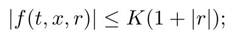
For any T > 0, assume that the coefficients f = f(t,x,r),g = g(t,x,r),σ = σ(t,x,r) in(1.1) are Borel functions of (t,x,r) ∈ [0,T]× [0,1]× R and that there exist positive constants K,L satisfying the following conditions:

(H1) for all (t,x,r)∈ [0,T]×[0,1]×R, it holds that

(H2) the function g is of the form g(t,x,r) = g1(t,x,r)+g2(t,r), where g1and g2are Borel functions satisfying that

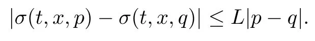
(H3) σ is bounded and for any (t,x,p,q)∈ [0,T]×[0,1]×R2,

Furthermore, f and g are locally Lipschitz with a linearly growing Lipschitz constant, i.e.,

Definition 2.1(mild solution) A random field Uε= {Uε(t,x) : t ∈ [0,T],x ∈ [0,1]} is called a mild solution of (1.1) with initial condition η if Uε(t,x) is Ft-measurable, (t,x) →Uε(t,x) is continuous a.s., and

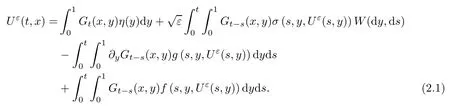
Here Gt(·,·) is the Green kernel associated with the heat operator ∂/∂t − ∂2/∂x2with the Dirichlet boundary conditions.

Foondun and Setayeshgar [9]proved the following result for the existence and uniqueness of the solution to eq.(1.1):

Theorem 2.1([9, Theorem 2.2]) Under conditions (H1)–(H3), for any η ∈ Lp([0,1]),p ≥2, there exists a measurable functional

Furthermore,from the proof of[9,Theorem 2.2],we know thatis bounded in probability, i.e.,

Particularly,taking ε=0 in(1.1),we know that the determinate equation(1.2)admits a unique solution U0∈C([0,T];L2([0,1])), given by

2.2 Main results

To study the CLT and the MDP, we furthermore suppose that

(H4) the coefficients f and g are differentiable with respect to the last variable, and the derivatives f′and g′are uniformly Lipschitz with respect to the last variable; more precisely,there exists a positive constant K′such that

for all (t,x)∈ [0,T]× [0,1],p,q ∈ R.

Combined with the growth condition (H3), we conclude that

Our first main result is the following functional central limit theorem:

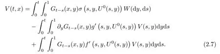
Theorem 2.2Under conditions (H1)–(H4), for any T > 0, the processconverges to a random field V in probability on C([0,T];L2([0,1])), determined by

The Cameron-Martin space associated with the Brownian sheet {W(t,x);t ∈ [0,T], x ∈[0,1]} is given by

The space H is a Hilbert space with inner product

The Hilbert space H is endowed with the norm

In view of the assumption (1.3) and (2.5), by the LDP for SPDE (see [6]), one can obtain that V/λ(ε) obeys an LDP on C([0,T];L2([0,1])) with the speed λ2(ε) and with the good rate function

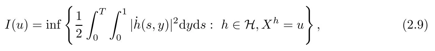
where the function Xhis the solution of the following deterministic partial differential equation:

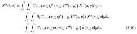
Our second main result reads as follows:

Theorem 2.3Under conditionsobeys an LDP on C([0,T];L2([0,1])) with the speed λ2(ε) and with the rate function I given by (2.9).

3 Some Preliminary Estimates

3.1 Some preliminary estimates

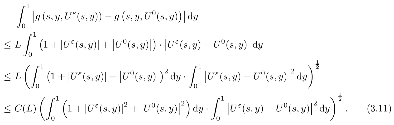
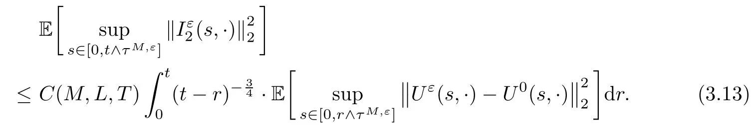
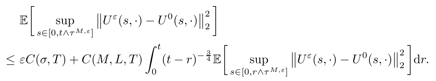
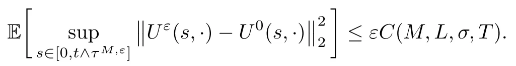
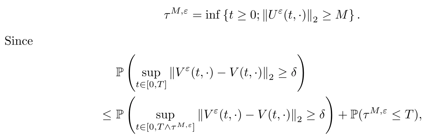
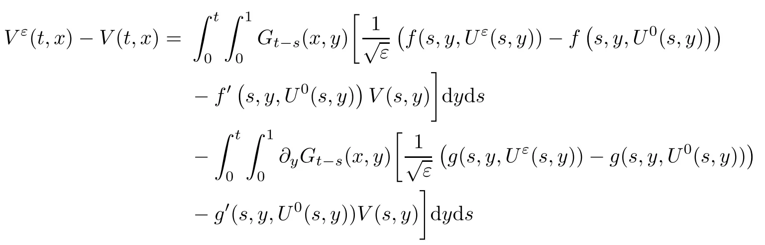
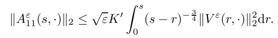
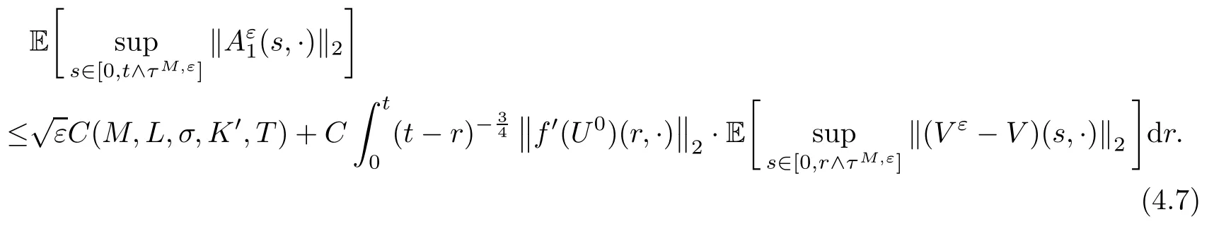
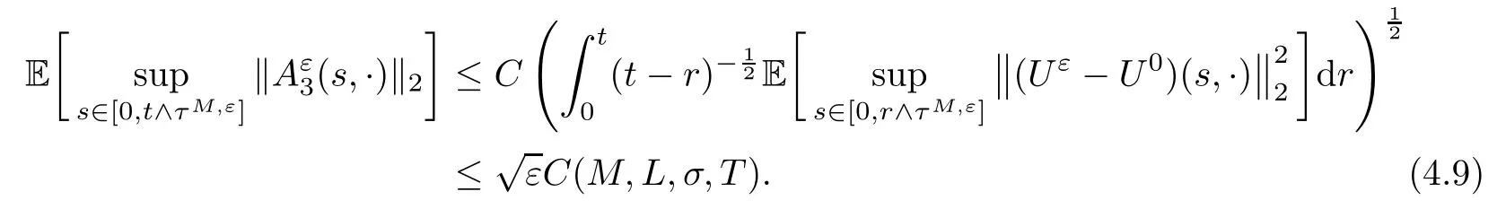
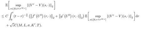
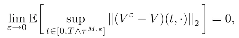
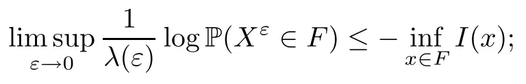
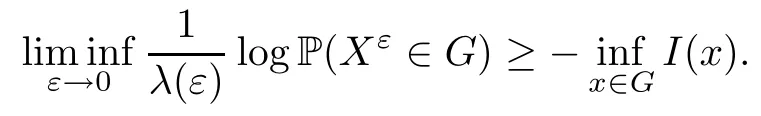
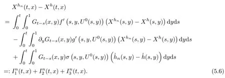
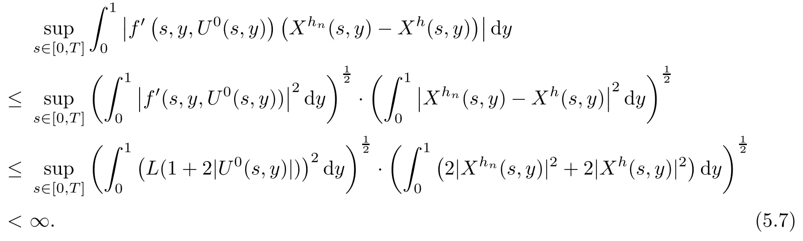
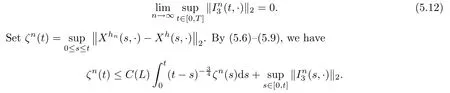
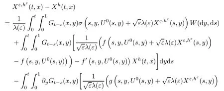
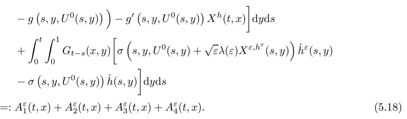
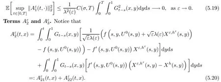
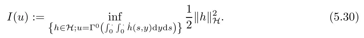
The following estimates of Green function G hold (see Cardon-Weber [6], Walsh [20],Gyngy [15]): there exist positive constants K,a,b,d such that for all x,y ∈ [0,1]and 0 ≤s

where ρ is the Euclidean distance in [0,T]× [0,1].

For any v ∈ L∞([0,T];L1([0,1])),t ∈ [0,T],x ∈ [0,1], let J be a linear operator defined by

Lemma 3.1([15, Lemma 3.1]) For any ρ ∈ [1,∞],q ∈ [1,ρ],K := 1+ 1/ρ − 1/q, it holds that J is a bounded linear operator from Lγ([0,T];Lq[0,1])into C([0,T];Lρ[0,1])for any γ >2K−1. Moreover,J satisfies the following inequalities:

(1) For every t ∈ [0,T]and γ >2K−1,

(2) For every 0< α (K/2 − α)−1, there exists a constant C >0 such that for all 0 ≤ s ≤ t ≤ T,

3.2 The convergence of Uε

This section is concerned with the convergence of Uεto U0as ε → 0.

For any M >0, define the stopping time

By (2.2), we know that

Proposition 3.2Under conditions (H1)–(H3), there exists some constant C(M,L,σ,T)depending on M,L,σ,T such that

ProofSince

by (H3) and Cauchy-Schwarz’s inequality, we have that for any (t,x)∈ [0,T]× [0,1],

Hence, applying Lemma 3.1 with ρ =2,q =1, and by Cauchy-Schwarz’s inequality, we have

First taking the supremum of time over [0,t ∧ τM,ε], and then taking the expectation, by the definition of τM,εwe obtain that

where we have used Fubini’s theorem in the last inequality.

Putting (3.10), (3.12), (3.13) and (3.14) together, we have

By Gronwall’s inequality (see [23]), we know that there exists a constant C(M,L,σ,T) such that

The proof is complete.

4 Proof of the Theorem 2.2

Proof of Theorem 2.2LetWe will prove that for any δ >0,

Recall the stopping time defined by

to prove (4.1) by (3.8), it is sufficient to prove that for any M >0 large enough,

By the definition of Vεand V, we have

By Taylor’s formula, there exists a random field ηεtaking values in (0,1) such that

Since f′is Lipschitz continuous, we have

If we frist take the supremum of s over[0,t∧τM,ε],and then take the expectation,by Proposition 3.2 we have

By first taking the supremum of s over [0,t ∧ τM,ε], and then taking the expectation, we have

Using (4.5) and (4.6), we have

For the term A3, by first taking the supremum of time over [0,t ∧ τM,ε], and then taking the expectation, by Burkholder’s inequality for stochastic integrals against Brownian sheets(see [16]), the Lipschitz continuity of σ and Proposition 3.2, we have

Putting (4.3) and (4.7)–(4.9) together, we have

By Gronwall’s inequalities ([23, Theorem 1]), (2.4) and (2.6), we have

which implies (4.2).

The proof is complete.

5 Proof of the Theorem 2.3

5.1 Weak convergence approach in LDP

First, recall the definition of a large deviation principle (c.f.[7]). Let (Ω,F,P) be a probability space with an increasing family {Ft}0≤t≤Tof the sub-σ-fields of F satisfying the usual conditions. Let E be a Polish space with the Borel σ-field B(E).

Definition 5.1A function I : E → [0,∞]is called a rate function on E, if for each M < ∞, the level set {x ∈ E : I(x) ≤ M} is a compact subset of E. A family of positive numbers {λ(ε)}ε>0is called a speed function if λ(ε)→ +∞ as ε → 0.

Definition 5.2{Xε}is said to satisfy the large deviation principle on E with rate function I and with speed function {λ(ε)}ε>0, if the following two conditions hold:

(a) (Upper bound) For each closed subset F of E,

(b) (Lower bound) For each open subset G of E,

Let A denote the class of real-valued{Ft}-predictable processes φ belonging to H a.s.,and let

The set SNendowed with the weak topology is a Polish space. Define

Recall the following result from Budhiraja et al. [5], which is based on certain variational representations for infinite dimensional Brownian motions ([2, 3]):

Theorem 5.1([5, Theorem 7]) For any ε > 0, let Γεbe a measurable mapping from C([0,T]× [0,1];R) into E. Suppose that {Γε}ε>0satisfies that there exists a measurable map Γ0:C([0,T]×[0,1];R)−→ E such that

(a) for any N <+∞ and family {hε}ε>0⊂ ANsatisfying that hεconverge in distribution as SN-valued random elements to h as ε → 0,converges in distribution to

(b) for every N <+∞, the setis a compact subset of E.Then the family {Γε(W)}ε>0satisfies an LDP in E with the rate function I given by

with the convention inf ∅ = ∞.

5.2 The skeleton equation

The purpose of this part is to study the skeleton equation, which will be used in the weak convergence approach.

Recall the skeleton equation defined in (2.10). Using the same strategy as that in the proof of the existence and uniqueness of the solution to eq.(1.1), we can state

Proposition 5.2Under conditions (H1)–(H4), eq.(2.10) admits a unique solution in C([0,T];L2([0,1])) satisfying that

For any h ∈H, set

where Xhis the solution of (2.10).

Theorem 5.3Under conditions (H1)–(H4), the mapping SN∋ h → Xh∈ C([0,T];L2([0,1])) is continuous with respect to the weak topology.

ProofLet {h,(hn)n≥1} ⊂ SNsuch that for any g ∈ H,

We need to prove that

Notice that

By Cauchy-Schwarz’s inequality, (2.4), (2.6) and (5.2), we have

Similarly, we obtain that

Since σ is bounded, for any fixed (t,x)∈ [0,T]×[0,1],the function Gt−s(x,y)σ(s,y,U0(s,y)):(s,y) ∈[0,t]×[0,1]→R belongs to L2([0,T]×[0,1];R). Asweakly in L2([0,T]×[0,1];R), it holds that

For any 0 ≤ s ≤ t ≤ T, applying formulas (3.5) and (3.6), by the boundness of σ and Hlder’s inequality, we obtain that

In particular, taking s=0, we obtain that

Hence, by a generalized Gronwall lemma (eg. [23, Theorem 1]), we have

which, together with (5.12), implies the desired estimate (5.5).

The proof is complete.

5.3 The controlled equation

This equation admits the unique strong solution

where Γεstands for the solution functional from C([0,T]× [0,1];R) into C([0,T];L2([0,1])).

The following lemma is a direct consequence of Girsanov’s theorem (refer to [9, Theorem 3.2]):

Lemma 5.4For every fixed N ∈ N, let h ∈ ANand Γεbe given by (5.14). Then Xε,h:= Γε(W + λ(ε)h)∈ C([0,T];L2([0,1])) solves the following equation:

Furthermore, by a similar calculation to that of [19, Lemma 5.2], we know that

Proposition 5.5Assume(H1)–(H4). For every fixed N ∈ N,let hε,h ∈ ANbe such that hεconverges in distribution to h as ε → 0. Then

in C([0,T];L2([0,1])) as ε → 0, where Γεand Γ0are given by (5.14) and (5.3), respectively.

ProofBy the Skorokhod representation theorem, there exists a probability basisand, on this basis, a sequence of independent Brownian sheetsand a family of F¯t-predictable processesbelonging totaking values on SN,such that the joint law of (hε,h,W) under P coincides with that ofunderand

From now on, we drop the bars in the notation for the sake of simplicity. Notice that

Term. Since σ is bounded, by Burkholder’s inequality for stochastic integrals against Brownian sheets (see [16]), we have

By Taylor’s formula, there exists a random field ηε(s,y) taking values in (0,1) such that

Since f′is Lipschitz continuous, we have

Define the stopping time

where M is some constant large enough.

Taking the supremum of time over[0,t∧τM,ε],and then taking the expectation,we obtain that

Putting (5.21) and (5.22) together, we have

In a fashion similar to the proof of (5.23), we obtain the following estimate for:

Using the same argument as that in the proof of (5.12), we obtain that

By the Lipschitz continuity of σ, we know that

By first taking the supremum of t over[0,T ∧τM,ε],and then taking the expectation,we obtain that

According to (5.25)–(5.27), we have that

Putting (5.18), (5.19),(5.23),(5.24)and(5.28)together,and by Gronwall’s inequality([23,Theorem 1]), we have

By Chebychev’s inequality, we have

Letting M →∞, by (5.16) we get the desired result (5.17).

The proof is complete.

5.4 The proof of Theorem 2.3

We are now ready to prove our main result. Recall the mapping Γ0given by (5.3). For any u ∈C([0,T];L2([0,1])), let

Proof of Theorem 2.3According to Theorem 5.1, we need to prove that the following two conditions are fulfilled:

(a) the set {Xh;h ∈SN} is a compact set of C([0,T];L2([0,1])), where Xhis the solution of eq.(2.10);

(b) for any family {hε}ε>0⊂ ANwhich converges in distribution as ε → 0 to h ∈ ANas SN-valued random variables, we have that

as C([0,T];L2([0,1]))-valued random variables, where Xhdenotes the solution of eq.(2.10)corresponding to the SN-valued random variable h (instead of a deterministic function).

Condition(a)follows from the continuity of the mapping SN∋ h → Xh∈ C([0,T];L2([0,1])),which was established in Theorem 5.3. The verification of condition(b)is given by Proposition 5.5.

The proof is complete.

AcknowledgementsWe would like to express our appreciation for R.Belfadli,L.Boulanba and M.Mellouk. They told us about their work on the stochastic Burgers’equation and pointed out a mistake in our paper.