Adelkader SAADALLAH Hamid BENSERIDI Mourad DILMI

Applied Mathematics Laboratory, Department of Mathematics, Faculty of Sciences,University of Ferhat Abbas- S´etif 1, 19000, Algeria

E-mail: saadmath2009@gmail.com; m benseridi@yahoo.fr; mouraddil@yahoo.fr

Abstract The goal of this article is to study the asymptotic analysis of an incompressible Herschel-Bulkley fluid in a thin domain with Tresca boundary conditions. The yield stress and the constant viscosity are assumed to vary with respect to the thin layer parameter ε.Firstly, the problem statement and variational formulation are formulated. We then obtained the existence and the uniqueness result of a weak solution and the estimates for the velocity field and the pressure independently of the parameter ε. Finally, we give a specific Reynolds equation associated with variational inequalities and prove the uniqueness.

Key words Asymptotic approach; Herschel-Bulkley fluid; Reynolds equation; Tresca law

1 Introduction

The subject of this work is the study of the asymptotic analysis of a generalized non-Newtonian fluid in a three dimensional thin domain Ωε. The contact boundary conditions considered here are the mixed and the friction law is the Tresca type.

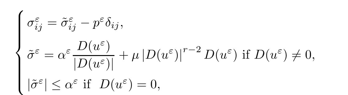
Herschel-Bulkley fluid is a generalized model of a non-Newtonian fluid which is introduced for the first time in 1926. In this work, we consider a thin film Ωεof R3during a time interval[0,T]. The equations that govern the stationary flow are as follows:

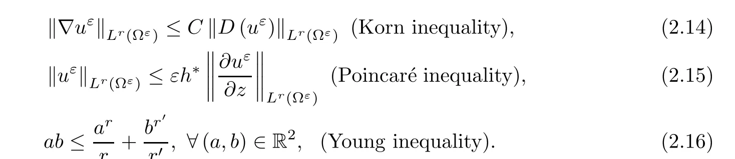
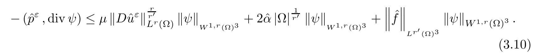
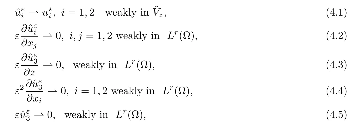
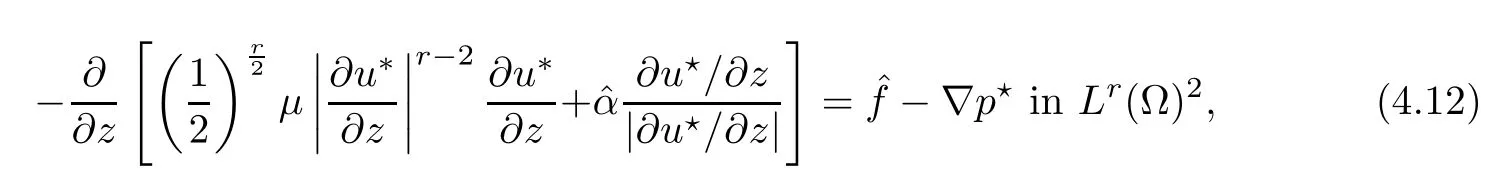
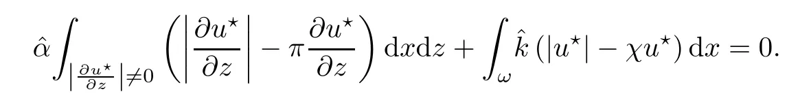
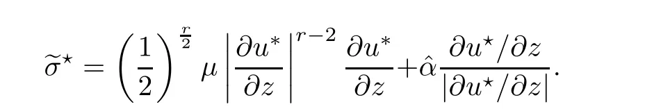
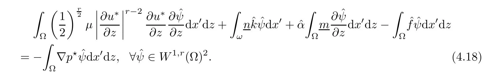
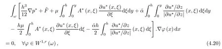
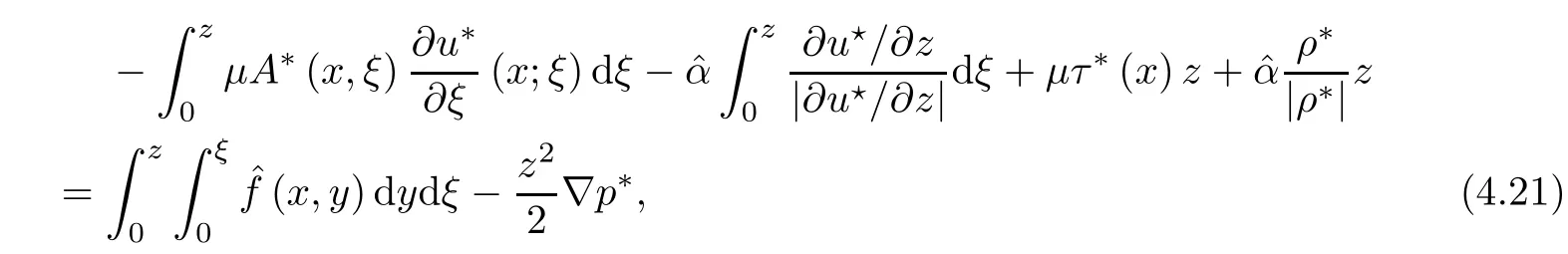
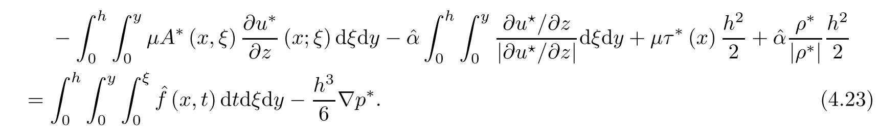
where αε≥0 is the yield stress, µ > 0 is the constant viscosity, uεis the velocity field, δijis the Kronecker symbol, 1

In many problems, which study the asymptotic behavior for a problem of continuum mechanics in a thin domain, we transform the problem into an equivalent problem on a domain Ωindependent of the parameter ε. Many research papers were written for similar problems with the same friction boundary conditions, however, these papers were restricted to the particular case of the considered problem. Let us mention some of the works done in [2, 3, 6]. In these articles, the authors consider a problem describing the motion of an incompressible Newtonian and non-Newtonian fluid in a three-dimensional thin domain flow with a non-linear Tresca interface condition. The asymptotic analysis of a Bingham fluid in a three dimensional bounded domain with Fourier and Tresca boundary conditions are also studied in [5]. Other contexts and problems can be found in the monographs such as in [9, 12, 13, 16], and in the literature quoted within. The numerical solutions of the Herschel-Bulkley fluid flow problems are studied in, for example, [8, 10, 11]. On the other hand, it is clear that the asymptotic analysis is valid for all the problems of continuum mechanics; the authors in [1, 14] studied the asymptotic analysis of a stationary and dynamical problem of non-isothermal elasticity with friction.

This article is organized as follows. First,in Section 2,we formulate and prove the existence and uniqueness results for the weak solution of the stationary equations for Herschel-Bulkley fluid in a three dimensional bounded domain with Tresca boundary conditions. In Section 3,we establish some estimates and convergence theorem. To this aim, we use the change of variable,to transform the initial problem posed in the domain Ωεinto a new problem posed on a fixed domain Ω independent of the parameter ε. Finally,the a priori estimate allows us to pass to the limit when ε tends to zero,then we prove the convergence results and limit problem with a specific weak form of the Reynolds equation,the uniqueness of the limit velocity distributions,and two-dimensional constitutive equation of the model flow considered.

2 Mathematical Formulation

We consider a mathematical problem governed by the stationary equations for Herschel-Bulkley fluid in a three dimensional bounded domain Ωε⊂R3with boundary Γε. This boundary of the domain is assumed to be composed of three portions: ω the bottom of the domain,the upper surface, and ΓεLthe lateral surface. The fluid is supposed to be incompressible. We impose a non-linear Tresca interface condition at the bottom and Dirichlet boundary conditions on the top and the lateral parts. The fluid is acted upon by given body forces of density f.

Let ω be a fixed region in the plane x=(x1,x2)∈R2. We suppose that ω has a Lipschitz boundary and is the bottom of the fluid domain. The upper surfaceis defined by x3=εh(x),where(0<ε<1)is a small parameter that will tend to zero and h is a smooth bounded function such that 0

We denotes by σεthe deviatoric part and pεthe pressure. The fluid is supposed to be viscoplastic, and the relation between σεand D(uε) is given by

For any tensor D = (dij), the notation |D| represents the matrix norm:

We denote by n=(n1,n2,n3)the unit outward normal vector on the boundary Γε. The normal and the tangential velocity on the boundary ω areSimilarly, for a regular stress tensor field σε, we denote byandthe normal and tangential components of σεon the boundary ω given by

We consider now the following mechanical problem.

Problem 1Find a velocity field uε:Ωε→R3and the pressure pε, such that

The law of conservation of momentum is given by equation (2.1). Equation (2.2) represents the constitutive law of a Herschel-Bulkley fluid, where 1 < r < 2 is the power law exponent of the material. Equation (2.3) represents the incompressibility equation. Equation (2.4) give the velocity on. As there is no-flux condition across ω, then we have equation (2.5).Condition (2.6) represents a Tresca thermal friction law on ω, where kεis the friction yield coefficient.

To get a weak formulation, we consider the following spaces:

A formal application of Green’s formula, using (2.1)–(2.6), leads to

Problem 2Find a velocity fieldandsuch that

where

ProofMultiplying equation (2.1)by (ϕ −uε), where ϕ ∈Kεand using Green’s formula,we get

According to the boundary conditions, we find

In (2.12), we add and subtract the termand obtain

Set

then

However, the condition of Tresca (2.6) is equivalent to

So,

Otherwise,

Let us deduce the following inequality

Using the Cauchy-Schwartz inequality, we obtain (2.7).

Theorem 2.1Assume that fε∈Lr′(Ωε)3and kε∈(ω); then there exists a unique solution (uε,pε) in(with additive constant) to the problem (2.7).

ProofWhen the functions test belong to, we obtain the variational problem: Find u ∈such that

This problem is still written as follows: Find u ∈such that

where

• a(uε,ϕ −uε) is bounded coercive hemicontinuous and strictly monotone [8].

• The proof of the existence of pεin Lr′0 (Ωε) with (uε,pε) satisfying (2.7) is given in [15].

We introduce some results which will be used in the next. The detailed description can be found in [2].

Theorem 2.2Let uεbe a solution of the variational inequality (2.7), then

ProofChoosing ϕ=0 as test function in inequality (2.7), we get

Using inequality (2.15), we have

By inequality (2.15)–(2.16), we have

From (2.18)–(2.20), we deduce (2.17).

3 Problem in Transpose Form and Some Estimates

In this section,we will use the technique of scaling in Ωεon the coordinate x3by introducing the change of the variables. We obtain a fixed domain Ω which is independent of ε:

Let us assume the following:

Let

where the condition(D′)is given by

By injecting the new data (3.1)–(3.2) into (2.7), then multiplying the deduced variational inequality by εr−1, we obtain

where

Now, we establish the estimates and convergences for the velocity fieldand the pressurein the domain Ω.

Theorem 3.1Let∈Kdiv(Ω)×(Ω) be the solution of variational problem(3.3), then there exists a constant C independent of ε such that

ProofMultiplying (2.17) by εr−1, we deduce

From Korn’s inequality and (3.5), there exists a constant CKindependent of ε, such that

From (3.6), we deduce (3.4), with, and

Theorem 3.2Under the same assumptions as in Theorem 3.1, there exists a constant C′independent of ε such that

ProofFor getting the first estimate on the pressure in(3.7)–(3.8),then in(3.3),choosing, we obtain

then

Using Hölder formula, we get

In a similar manner, in (3.3) we choose, then we obtain

From (3.9) and (3.10), we have

When i=1,2, we choose ψ =(ψ1,0,0), then ψ =(0,ψ2,0), in inequality (3.11), we obtain

where C1= µC and |Ω| = mes(Ω). Then, (3.7) follows for i = 1,2. For getting (3.8), by inequality (3.11), and ψ =(0,0,ψ3), we find

4 Convergence Results and Limit Problem

Theorem 4.1Under the same assumptions as in Theorem 3.1,there existandsuch that

For the proof of Theorem 4.1, we follow the same steps as in [4].

Theorem 4.2With the same assumptions of Theorem 4.1, the solution (u∗,p∗) satisfy the following relations

The proof of this theorem is based on the following lemma.

Lemma 4.3(Minty) Let E be a reflexive Banach space,A be a nonempty closed convexe subset of E, and E′be the dual of E. Let T: A →E′be a monotone operator which is continuous on finite dimensional subspaces (or at least hemicontinuous). Then, the followings are equivalent:

ProofUsing Minty’s Lemma 4.3 and the fact that div(ˆuε) =0 in Ω, then (3.3) is equivalent to

Using Theorem 4.1 and the fact that j0is convex and lower semi-continuous, (lim inf j0()≥j0(u∗)), we obtain

Using again Minty’s Lemma for the second time, then (4.8) is equivalent to (4.7).

Theorem 4.4The variational inequality (4.7) is equivalent to the following system

and

ProofChoosing=2u⋆and=0 respectively in (4.7), we obtain (4.9).

Theorem 4.5Set

then

where π is obtained in the proof.

ProofIf, from (4.11) we get. For all, choosingthenin (4.10), we obtain

where

Now,utilising the Hanh-Banach theorem,then,∃(χ,π)∈L∞(ω)2×L∞(Ω)2,with, such that

In particular, from (4.9) and (4.14), we get

Also, from (4.13) and (4.14), we have

Now using (4.15), we have

Besides, from (4.16), there exists p⋆∈Lr′(Ω) such that

Using (4.17)–(4.18) becomes

In the following theorem, we give the convergence of our problem towards the Reynolds equation.

Theorem 4.6Under the assumptions of preceding theorems, u⋆and p⋆satisfy the following equality

where

ProofTo prove (4.20), integrating twice (4.13) between 0 and z, we obtain

Integrating (4.22) between 0 and h, we get

From (4.22), we deduce

By (4.23) and (4.24), we obtain

Therefore, for ϕ ∈W1,r(ω), we deduce (4.20).

Theorem 4.7The solution (u∗,p∗) inof inequality (4.7) is unique.

ProofLet(u∗,1,p∗,1)and(u∗,2,p∗,2)be two solutions of (4.7); taking ϕ = u∗,2and ϕ=u∗,1respectively, as test function in (4.7), we get

Observe that for every x,y ∈Rn,

we obtain

From (4.25) and (4.26), we deduceFinally, to prove the uniqueness of the pressure, using equation (4.20) with the two pressures p∗,1and p∗,2, we find

Taking ϕ = p∗,1−p∗,2, and by Poincar´e inequality, we deduce. So,

AcknowledgementsThe authors thank Prof. El-Bachir Yallaoui for his help in revising the English language in the article.