Meng-de Zhng , Hi-f Di ,*, Bi-qing Hu , Qi Chen

a College of Electrical Engineering, Naval Univ. of Engineering, Wuhan 430033, China

b Qingdao Brigade, Shandong Branch of the Armed Police Marine Police Corps, Qingdao 266033, China

Keywords:Integrated navigation Support vector regression Unscented Kalman filter Robust filter Adaptive filter

ABSTRACT Aiming at the problem that the traditional Unscented Kalman Filtering (UKF) algorithm can’t solve the problem that the measurement covariance matrix is unknown and the measured value contains outliers,this paper proposes a robust adaptive UKF algorithm based on Support Vector Regression (SVR). The algorithm combines the advantages of support vector regression with small samples, nonlinear learning ability and online estimation capability of adaptive algorithm based on innovation.Firstly,the SVR model is trained by using the innovation in the sliding window, and the new innovation is monitored. If the deviation between the estimated innovation and the measured innovation exceeds a given threshold,then measured innovation will be replaced by the predicted innovation, and then the processed innovation is used to calculate the measurement noise covariance matrix using the adaptive estimation algorithm. Simulation experiments and measured data experiments show that SVRUKF is significantly better than the traditional UKF, robust UKF and adaptive UKF algorithms for the case where the covariance matrix is unknown and the measured values have outliers.

1. Introduction

Strapdown inertial navigation System(SINS) has the characteristics of simple structure, small size, light weight, comprehensive output navigation information and good autonomy. It has become the focus of research.However,the SINS has the same problem that the navigation accuracy diverges with time as with the platform inertial navigation system.It cannot correct error relying on its own[1-3], such that it requires combined navigation. The strapdown inertial base integrated navigation system is a system that corrects navigation information using strapdown inertial navigation and another or more non-similar navigation systems [4,5]. Common Strapdown Inertial Navigation System can be applied to land navigation (GPS, odometer), underwater navigation (Doppler Velocity Log, DVL) [2,3,6,7]. However, the key technology of the integrated navigation is the filtering method [2].

In 1960, R.E. Kalman proposed the Kalman filtering (KF) algorithm [8], which became the cornerstone of integrated navigation research in recent decades.However,the classical KF can only solve the linear state estimation problem. In 1995, S. J. Julier and J. K.Uhlmann proposed the Unscented Kalman filter (UKF) [9], which has a higher estimate and stability in nonlinear systems and become a research hotspot [10-12]. In the practical application of strapdown inertial base integrated navigation, the accuracy and real-time of estimation are both problems to be considered. The less computational complexity and higher precision of UKF make it a feasible nonlinear filtering method which is widely used in navigation[13,14].This is an important reason for its research hotspot.In 2003, Crassidis first proposed a quaternion-based UKF for spacecraft attitude estimation, known as unscented quaternion estimator (USQUE) [10]. In Ref. [15], the USQUE algorithm for quaternion expression attitude is improved, which reduces the computational complexity of USQUE. The method is applied to SINS/GPS direct integrated navigation. Zhou J, Edwan E et al. [16]studied the application of USQUE for tightly integrated MEMS and GPS navigation system.In Ref.[17],the performance of UKF,MEKF and KF in MEMS/GPS system are compared. The results show that UKF has the highest accuracy and the largest amount of calculation.

In the practical application of strap-down inertial base integrated navigation, the SINS itself is relatively stable and is not susceptible to interference and thus affects system noise. The environmental conditions are complex and changeable, which makes it difficult to avoid pollution and interference,which in turn affects the measurement noise covariance matrix. The polluted measurements will have a greater impact on the accuracy of the UKF. The computed covariance matrix is not always guaranteed to be positive definite because of the negative sigma points which even lead to the divergence of the filter[11,18-20].For example,if a SINS/GPS system is used in a city, there may be cases where the satellite signals are blocked or interfered[21]; when the SINS/DVL system is used underwater, there may be problems such as abnormal water velocity caused by changes in water flow rate or bottom geography [22]. How to improve the anti-interference ability of the algorithm is a problem that the UKF must solve in practical applications.In Ref.[23],a robust algorithm based on the Mahalanobis distance (MD) method is proposed, which can improve the robustness of KF,but it cannot be applied to nonlinear systems.In Ref.[11],Huber’s robustness method is extended to UKF to estimate position, velocity and constant which achieves the robustness of UKF for integrated INS/GPS. In addition, an accurate priori measurement covariance matrix is often difficult to obtain,and may change with the motion state and environment. Robust methods alone do not yield optimal results. Therefore, the literature [24] proposed an adaptive UKF filtering algorithm based on sliding window, which improves the adaptive ability of the UKF algorithm, but does not consider the possibility that there may be outliers in practical applications.In Ref.[25],a robust adaptive UKF filtering method based on innovation and residuals is proposed for the simultaneous existence of outliers and uncertain covariance matrices. However, in this method, the method of reducing the weight of outliers is used. It will still be affected by the wild value and the filtering accuracy will decrease.

Aiming at the above problems, this paper proposes a robust adaptive UKF method based on SVR, which can automatically detect outliers and replace the current innovation with real-time estimated innovation instead of reducing the weight of wild value. The algorithm enhances the anti-jamming capability of the algorithm without reducing the filtering accuracy.

The organization of this paper is as follows. In the review of existing theories, the basic SINS equations and USQUE are introduced. In the introduce of the SVRUKF section, this section first extend the Innovation-based adaptive estimation(IAE)to nonlinear filter case within UKF framework. The principle of improving the robustness of SVR is studied. Then SVRUKF are derived in detail.Finally, simulation testing and ship-borne experiments were conducted and are summarized in the experimental section. The results are provided and the performance of the traditional methods and SVRUKF are compared. The experimental results show that SVRUKF is superior to the traditional robust algorithm and adaptive algorithm.

2. Theoretical review

2.1. SINS basic equations

The quaternion kinematics equation is given by

So, the SINS basic equations using ENU coordinate with the quaternion are summarized.

where,

where, ωieis the Earth’s rotation rate are given as (from WGS-84)7.292115×10-5rad/sec. and

where, λ is the latitude a = 6378137m, e = 0.0818. The g is local gravity (from WGS-84) are given as approximately 9.8 m/s2.

The gyro measurement model is given by

where, ε is gyro bias, ηgvand ηguare zero-mean Gaussian whitenoise process.

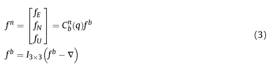
integrated navigation system is shown in Fig. 2. The accelerometer measurement model is given by

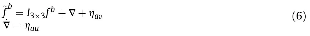
where,∇is accelerometer bias,ηavand ηauare zero-mean Gaussian white-noise process.

Fig.1. USQUE algorithm.

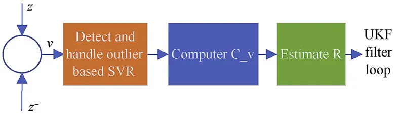
Fig. 4. The innovation process in the adaptive SVRUKF.

2.2. USQUE

Because UKF cannot be directly applied to the strap-down inertial base integrated navigation system with quaternion expression attitude,it is difficult to guarantee that the attitude quaternion parameter normalization constraint problem and the quaternion filtering variance matrix matching constraint problem are difficult to guarantee. USQUE solves the problem of UKF’s attitude estimation in the equation of state through“layered filtering”.The filtering process is divided into two layers,the inner layer filtering uses the generalized error Rodrigues parameter to update the attitude state,and the outer layer filtering uses the quaternion to perform the attitude state transfer. The quaternion and generalized error Rodrigues parameters use the attitude transformation relationship of multiplicative error quaternions as a bridge for switching. The basic idea of USQUE is shown in Fig.1, and the algorithm flow is shown in Algorithm 1-3.

The following is the derivation of the filtering process of USQUE combined with the strapdown inertial base integrated navigation system. The equation of state has been described in detail above.Similar to MEKF [23], the state quantity is divided into two parts:attitude quantity and non-attitude quantity.The non-attitude part is seen in MEKF algorithm,and the attitude part is error Rodrigues parameteris the other states used in SINS/GPS system. The state vector is=The corresponding filter variance matrix is Pk-1.

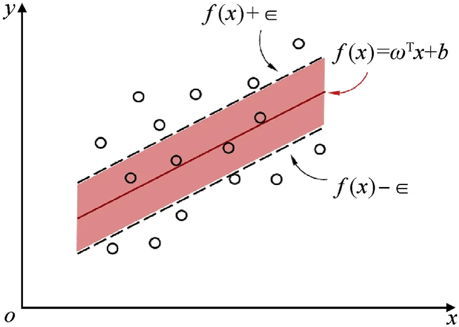
Fig. 3. Support vector regression diagram.

USQUE algorithm is estimated byand Pk-1according to the state estimate. Determine the corresponding quaternion attitudeIn the measurement update,the measurement equation is nonlinear if the tight couple or super-tight couple is adopted. For the USQUE algorithm,the measurement update process is basically the same as the time update. In the loose couple method, the measurement equation is a linear equation. Since the attitude is represented by the Rodrigues parameter,the measurement update process is the same as KF. After the measurement update is completed,the attitude expressed by the Rodriguez parameter will be used by, converted to quaternion, This is the purpose of the attitude update. This paper introduces the measurement update by taking the loose couple as an example.

Among them, depending on the measurement, Hkis different.

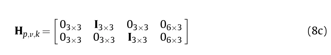
When only the position is used as the external aiding information, the measurement matrix is:

When only the velocity is used as the external aiding information, the measurement matrix is:

When the position and velocity are used as the external aiding information, the measurement matrix is:

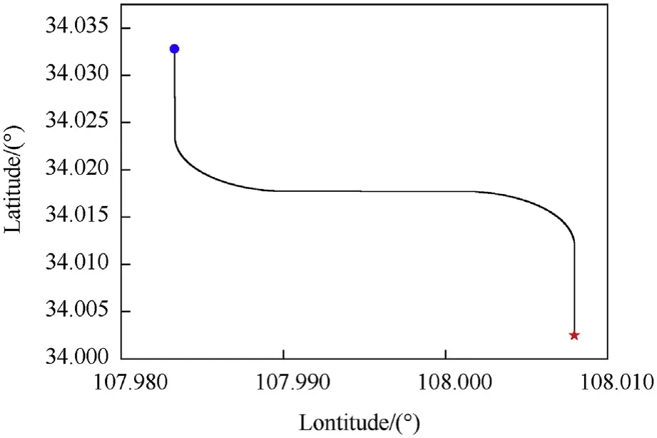
Fig. 5. Simulation trajectory.

Time Propagation:Define the filtering state Using error MRP describe attitude ^xk-1（δℜ） = [^xδℜk-1;^xε k-1]Using quaternion describe attitude ^xk-1（q）=[^xqk-1;^xε k-1] and covariance Pk-1#Create sigma points using UT χk-1（i） ="χδℜk-1（i）χε k-1（i）= sigma（^xk-1（δℜ），Pk-1）The χδℜk-1（i） corresponding quaternion error χδqk-1（i） = [δρk-1（i）;δq4，k-1（i）]δq4，k-1（i） =-a■■■χδℜk-1（i）■■■2+f■■■■■■■■■■■■■■■■■■■■■■■■■■■■■■■■■■■■■■■■■■■■■■■■■■■f2 +（1-a2）■■■χδℜk-1（i）■■■2 f2 +■■■χδℜk-1（i）■■■2 δρk-1（i） = f-1[a +δq4，k-1（i）]χδℜk-1（i）Compute the quaternion sigma points χqk-1（i）=χδqk-1（i）⊗^qk-1 then χk-1（i） = [χq k-1（i）;χek-1（i）]Propagate sigma points χk/k-1（i） = f（χk-1（i）） = [χq k/k-1（i）;χek/k-1（i）]Compute error quaternion sigma points χδq k/k-1]-1and χδqk/k-1（i） = [δρk/k-1（i）;δq4，k/k-1（i）]Compute GRP sigma points χδℜk/k-1（i）=f k/k-1（i）=χq k/k-1（i）⊗[x q δρk/k-1（i）a+δq4，k/k-1（i） and χk/k-1（i） = [χδℜk/k-1（i）;χek/k-1（i）]The predicted mean and covariance of state^xk/k-1 = ∑2n i=0 w（i）χk/k-1（i）Pk/k-1 = ∑2n i=0 w（i）（χk/k-1（i） - ^xk/k-1）（χk/k-1（i）-^xk/k-1）T + Wk-1 Measurement update:Compute filtering gain Kk = Pk/k-1HTk[HkPk/k-1HTk +Rk]-1 Compute posterior mean and covariance,^xk =^xk/k-1 +Kk（yk-Hk^xk/k-1） and ^xk =[^xδℜk-1;^xek]Pk =（In×n-KkHk）Pk/k-1 with In×n is n-dimension unit matrix Attitude update:The ^xδℜk corresponding quaternion is shown by^xδq k （i） = [δρk（i），δqk，4（i）]T With-a■■^xδℜ■■2+f■■■■■■■■■■■■■■■■■■■■■■■■■■■■■■■■■■■■■■■■■■■■f2 +（1-a2）■■■^xδℜ■■■2 δq4，k =k k k f2 +■■■^xδℜk■■■2 且δρk = f-1[a +δq4，k]^xδℜThe update of quaternion is given by^xqk = ^xδqk ⊗x k/k-1 and δℜk⇒0,^xk（q） = [^xqk;^xεk]then enter the next filtering cycle.q

2.3. SINS/GPS integrated navigation system

By using accelerometer measuring force and gyroscope measuring the angular rate, SINS can output attitude, velocity and position. Then attitude, velocity and position are entered into UKF time propagation as state. The position information provided by GPS is entered into UKF measurement update. Finally, the filter estimate is obtained (see Fig. 2).

3. Derivation of the SVRUKF

It is known that the standard UKF performs poorly when the measurement noise deviates from the assumed Gaussian model.In order to improve the performance of the standard UKF in the case without accurate noise model and/or with outliers,this section first extend the Innovation-based adaptive estimation(IAE)to nonlinear filter case within UKF framework, forming adaptive UKF(AUKF).Then the Support Vector Regression (SVR) algorithm is used to robust the AUKF, forming robust adaptive UKF(SVRUKF).

3.1. IAE-based UKF

3.1.1. IAE-based EKF

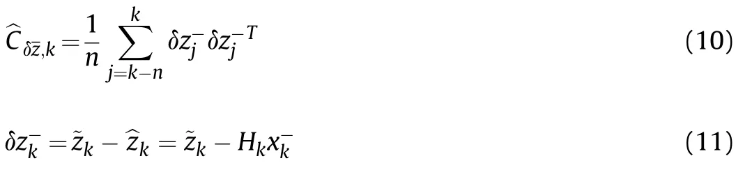
The Innovation-based adaptive estimation (IAE) algorithm is a method of calculating the system noise covariance Q,measurement noise covariance R,or simultaneously calculating Q and R from the observation information statistics. The method estimates the covariance matrix C of the observed information by the innovationin the sliding window of width n:

This can be used to calculate the measurement noise matrix R and the system noise matrix

3.1.2. AUKF

For the UKF, if the observation equation is linear, then the observation update is the same as the normal KF, so the system noise and the measurement noise covariance matrix can be adaptively estimated directly using the above formula.

If the observation equation is nonlinear,then the measurement update requires a UT transformation, and the predicted value is

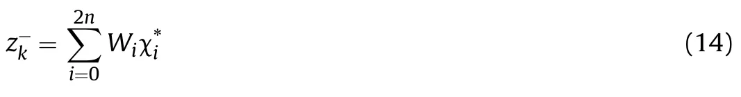
The calculation of the innovation will become

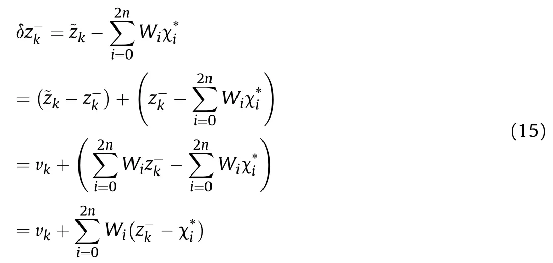
According to the central limit theorem, the innovation satisfies the zero mean Gaussian distribution. That is E（δz-k） = 0, so

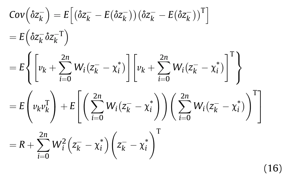
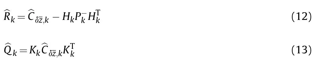
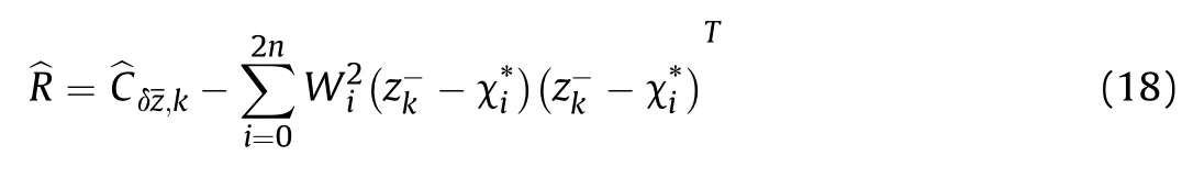
According to Eqs.(2)and(10),the estimated covariance matrix can be obtained as

3.2. Robustify the UKF

Due to the influence of the environment, the measurements of the sensor may have outliers.If these outliers are not processed,the covariance matrix estimated by the adaptive will seriously deviate from the true value,resulting in a decrease in filtering performance.Therefore,this section uses support vector regression to detect and process outliers.

3.2.1. Support vector regression

The principle of regression analysis using the support vector machine is to project the multi-dimensional nonlinear relation sample set into the high-dimensional feature space G through the nonlinear mapping x→Φ（x） to become a linear relationship, and then perform linear regression in this high-dimensional feature space. Given n data samples ｛xi，yi｝，i = 1，2，…，n, where xiis the actual observation and yiis the expected value. Use the following formula to estimate the regression function f21:

where,Φ（x）is the mapping function,b is the offset,ω is the vector in the high-dimensional feature space G, and Rnis the dimension real space.

As shown in Fig. 3, the goal of SVR regression is to find a hyperplane that causes the“distance”and minimum of sample points that fall outside the red region to the hyperplane. Consider the relaxation variable and regularization, get the cost function

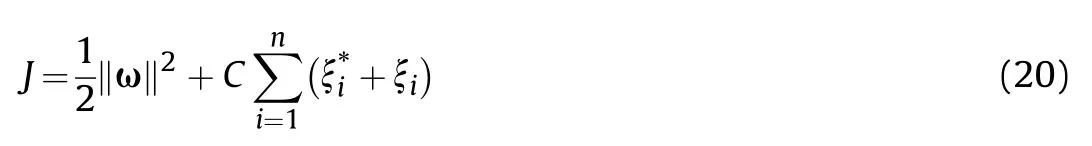
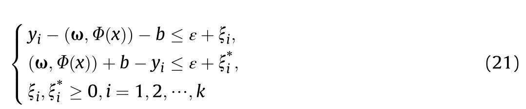
where,C is a penalty factor;ξiandare the relaxation factors,ε is a loss function.

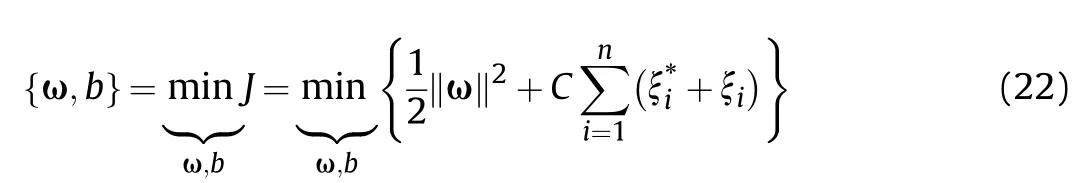
The goal of optimization is to solve the parameters ω and b to minimize the cost function

The above optimization model can be regarded as a quadratic programming problem, using the Lagrange dual form and introducing a kernel function expression, then equation (20) is transformed into:

The constraint is

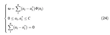
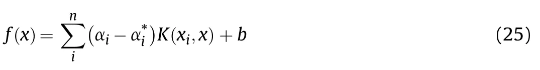
where αiandare the weighting coefficients of the support vector and K is the kernel function.By solving equation(20),αiandcan be obtained, and substituting equation (22) into equation (17) can obtain the solution of SVR.

The above process needs to satisfy the KKT condition (22)It can be seen from equation(24)that there is（C-αi）ξi=0 and αi（f（xi）-yi-ε-ξi）=0 for any one sample （xi，yi）. So, after getting αi, if 0 ＜αi＜C, there must be ξi= 0, so there is

3.2.2. Robust AUKF based on SVR

Let the innovation time series be ｛δz1，δz2，…δzt｝. These time series satisfy certain changes. However, since the innovation is generally multi-dimensional,the relationship between them is not a simple linear relationship,so it is difficult to use the conventional fitting method to establish this relationship model.

In her desire to please everyone she ceased to be sincere, and degenerated17 into a mere18 coquette; and even her lovers felt that the charms and fascinations19 which were exercised upon all who approached her without distinction were valueless, so that in the end they ceased to care for them, and went away disdainfully

If the current time data δzt+1is predicted based on the historical data of δzt,the mapping f:Rm→R:can be established to satisfy the(23)

Where m is the number of historical data used in the prediction function, i.e. the order of the model.

The model of support vector regression can be obtained by learning from the sample,so that the predicted value at the current moment is:

Calculate the difference between the predicted value and the actual measured value

The principle of determining the wild value is:

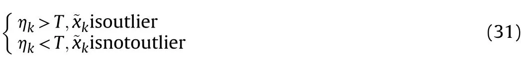
where, T is the threshold value. Regarding the selection of the threshold value, the literature [23] is selected according to experience and lacks theoretical basis. This paper combines the 3σ criterion to calculate the mean δ~z and standard deviation σδzof the innovation in the sliding window.

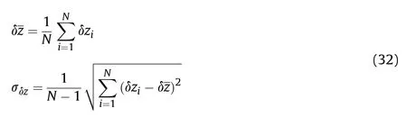
Further determining the threshold

If the measured value is judged to be a outlier (as long as a certain dimension in the innovation vector exceeds the threshold value and is determined to be a wild value), the predicted innovation is used to replace the original innovation, and the measurement update is completed. 百度翻译See Fig. 4 for the whole process.

The key to Kalman filter application in practice is to coordinate the contradiction between the algorithm in ideal state and the problems in practical application. It requires Kalman filter to solve practical problems through anti-interference processing. Robustness and adaptation are the methods to improve the anti-jamming ability of filtering.The traditional robust filter is mainly used to deal with the problem of system interference. Through the method of weighted, traditional robust filter reduce the variance of measurement noise. So, the anti-jamming ability of the filter is improved by using as little external information as possible. The essence is to reduce the filter gain matrix K.The adaptive algorithm is mainly used to deal with the degradation of filtering performance caused by inaccurate estimation of measurement noise covariance matrix. In this paper, SVRUKF is used to improve the estimation accuracy of robust filter and adaptive filter. What’s more, it can solve the problem of poor estimation effect of RUKF in the case of large outliers.The experimental part will prove the effectiveness of SVRUKF.

4. Simulation study and experiments

In this section,the investigated robust adaptive filtering method for the SINS integrated navigation is evaluated through simulation and ship-borne experiment. The simulation and ship-borne experiment used SINS/GPS loosely integration whose position as its measurement variables. Unlike MEMS, the most important navigation parameters of high accuracy SINS/GPS integrated navigation are yaw and position, especially in the field of marine navigation.Therefore,in this part,we will focus on the estimation error of yaw and position.From the analysis of the results,we are able to prove effectiveness of the SVRUKF (see Fig. 4).

4.1. Simulation study

The simulation produces a running track of the car(as shown in Fig. 5), and the simulation time is 680 s. The red pentagram indicates the initial position of the car,the blue solid circle indicates the end position of the car,the initial speed is 15 m/s,and the initial yaw is 0°. The sensor specification are shown in Table 1.

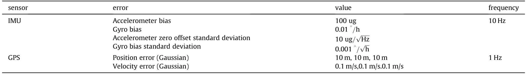
Table 1 Sensors specifications.

Set the initial conditions of the filter:horizontal error 0.5’, yaw error 30’,speed error in each direction 0.1 m/s,position error 10 m.The window size involved in the SVRUKF is 60 s. The CPU of computer is Intel Pentium CPU G4600 (3.60 GHz).

4.1.1. Case 1

The main purpose of this experiment is to test the performance of SVRUKF in inaccurate initial measurement noise covariance matrix. Set the initial covariance matrix R to 100 times the true value. The results obtained by the four methods of UKF, AUKF,HUKF, and SVRUKF, respectively, are shown in Fig. 6(a)-(c).

It can be seen from the two graphs in Fig. 6(a)-(b) that under the condition that the initial covariance matrix has large uncertainty, the positioning error and yaw error of the traditional UKF method and the robust UKF method do not converge to zero, the estimation accuracy decreases,and the AUKF and SVRUKF methods gradually converge around 80s and finally approach zero. This is because the latter two methods succeed in estimating the more accurate measurement covariance matrix in a shorter time. Make the estimation results optimal. Through the Frobenius norm comparison curve of the difference between the covariance matrix and the real covariance matrix estimated by the two adaptive methods in Fig. 6(c), it can be seen that the estimation accuracy of the two methods for the covariance matrix is comparable, but the method proposed in this paper has a faster convergence speed than the traditional adaptive method, which is 30 s and 60 s respectively.The position errors in Figs. 6, 7 and 9 are calculated from the distance between the longitude and latitude estimates and the reference values.

Table 2 shows the location and yaw Root mean square error(RMSE)tatistics and total computing time of the whole estimation process for different algorithms. As we all know, RMSE can well reflect the precision of measurement. The RMSE equation in Tables 2, 3 and 5 are given by:

It can be seen from Table 2 that the accuracy of the position and yaw error of the HUKF algorithms is about 2.73 m and 4.51’. The position estimation accuracy of the AUKF and SVRUKF algorithms is 1.71 m and 1.65 m.The performance of SVRUKF is 59%higher than the ordinary UKF.The yaw error of AUKF is worse than the ordinary UKF, and the yaw error of SVRUKF is reduced to 2.1’ which has a great improvement. The above analysis shows that SVRUKF can adaptively estimate the covariance matrix under the condition of covariance uncertainty, and the performance is better than the ordinary AUKF. In terms of computing time, UKF, AUKF and RUKF are almost equivalent at around 22 s. SVRUKF is 36.0250 s. When talking about average computational time of each integrated navigation update step, UKF is 33.2 ms, RUKF is 31.3 ms, AUKF is 33.9 ms, SVRUKF is 52.9 ms. Considering the practical application,we pay more attention to the effect of integrated navigation.Therefore, GPS update frequency is used as update frequency for calculation average computational time for each integrated navigation update step.SVRUKF takes more 19.7 ms per step than UKF.Because this period of time is very short,it is completely acceptable.

In the case of inaccurate measurement noise covariance matrix,RUKF improves anti-jamming capability by reducing filter gain matrix K. It will inevitably lead to a decline in the accuracy of estimation. SVRUKF is slightly better than AUKF. Some measurement noises can lead SVR to judging that filtering innovation is with outliers.So filtering innovation is replaced by prediction.This is the reason why SVRUKF improves the performance of adaptive filter.

4.1.2. Case 2

The main purpose of this experiment is to verify the performance of SVRUKF when the measurement contains large outliers and inaccurate measurement noise. Set the initial covariance matrix R to 100 times the true value, and add a field value of 1000 m every 60 s horizontal position. The results obtained by the UKF,AUKF, HUKF, and SVRUKF methods are shown in Fig. 7(a)-(b).

It can be seen from the graphs shown in Fig. 7(a)-(b) that UKF and AUKF are completely divergent under the condition of containing the outliers and the uncertain initial measurement noise covariance matrix, and HUKF can converge slowly due to the robustness to the wild value,and the SVRUKF method proposed in this paper can converge at a faster speed and the convergence accuracy is better than HUKF.

Table 3 shows the position RMSE,yaw RMSE statistics and total computing time of the whole estimation process for different algorithms. It can be seen from Table 3 that the positional errors of the UKF and AUKF algorithms are very large, 21 m and 16.9 m,respectively.HUKF is able to keep the position error at around 3 m,which is a big improvement.The SVRUKF method works best,with position error and yaw error of 1.93 m and 2.32’.The above analysis shows that SVRUKF can adaptively estimate the covariance matrix under the condition of outlier and covariance uncertainty,and the performance is better than the other three methods. When discussing computing time,UKF,AUKF and RUKF are almost equivalent at around 22 s. While, SVRUKF is 36.165 s. When talking about average computational time of each integrated navigation update step, UKF is 33.5 ms, RUKF is 32.2 ms, AUKF is 34.4 ms, SVRUKF is 53.1 ms.

According to the results of the experiments,when talking about estimation of position, UKF and AUKF have no ability to tolerate position outliers. HUKF has certain capability to tolerate outliers.However, SVRUKF is the best in terms of convergence speed and estimation accuracy. It proves that SVRUKF has better robustness than RUKF.So,SVRUKF has better solved the problem that RUKF is not good at dealing with large outliers.In yaw estimation,SVRUKF has the best estimation result because it can accurately estimate the correct value of outliers and estimate measurement noise covariance. The characteristics of RUKF sacrificing accuracy to improve anti-infective ability have been verified. Similarly, AUKF also has some anti-jamming ability. UKF also appear jagged in course estimation because of poor resistance to outliers.

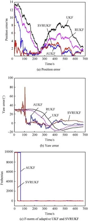
Fig. 6. Comparison of different algorithm results under unknown conditions of covariance matrix.

Fig. 7. Comparison of different algorithms with outliers and uncertain covariances.

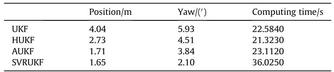
Table 2 Total computing time and RMSE of position and yaw.

Table 3 RMSE of position, yaw and total computing time.

4.2. Ship-borne experiment

This section verifies the SVRUKF proposed in this paper based on the ship-borne experimental data. The experimental data was collected from a ship-borne experimental system. The sensor configurations used in the shipboard experiments are shown in Table 4. The ship-borne experiment was carried out in theChangJiang River. The experimental process was designed as follows: When the experimental system was turned on, the test ship remained moored for about 15 min; then the test ship sailed out and the motion was about 6.4 h. The whole motion trajectory is shown in Fig. 8.

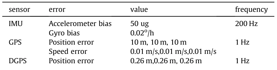
Table 4 Sensors specifications.

Table 5 Total computing time and RMSE of position and yaw.

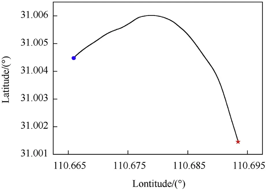
Fig. 8. Trajectory of the ship.

The data of 600 s was selected for experimental verification.For GPS data, add an outlier of 1000 m every 60 s horizontal position.Initial conditions:horizontal error 0.1°,yaw error 1°,using GPS data to initialize position and speed. SINS/GPS integrated navigation is implemented by four methods:UKF,AUKF,HUKF,and SVRUKF,and differential SINS/GPS is used as a benchmark. The window size involved in the SVRUKF is 60 s. The CPU of computer is Intel Pentium CPU G4600 (3.60 GHz). The results obtained are shown in Fig. 9(a)-(b).

It can be seen from the graphs shown in Fig. 9(a)-(b) that UKF and AUKF are completely divergent under the condition of containing the outlier and the uncertain initial covariance matrix,and HUKF can be slow converge due to the robustness to the outlier.And the SVRUKF method proposed in this paper can converge at a faster speed and the convergence accuracy is better than HUKF.

Fig. 9. Comparison of measured data filtering results.

Table 5 shows the position and yaw RMSE statistics and total computing time of the whole estimation process for different algorithms. It can be seen from Table 5 that the positional errors of the UKF and AUKF algorithms are very large, 21.88 m and 19.74 m,respectively. HUKF is able to keep the position error at around 3.89 m. The SVRUKF method works best, with position error and yaw error of 0.48 m and 2.16’. The above analysis shows that SVRUKF can adaptively estimate the covariance matrix under the condition of outlier and covariance uncertainty, and the performance is better than the other three methods. SVRUKF takes around 50 s more computing time than UKF. It is caused by the prediction filter innovation of SVR algorithm.The SINS’s frequency update of ship-borne experimental is 200 Hz, while the SINS’s frequency update of simulation test is 10 Hz. So, the calculation time of ship-borne experimental is far longer than simulation test.As for average computational time of each integrated navigation update step,UKF is 0.880 s,RUKF is 0.882 s,AUKF is 0.884 s,SVRUKF is 0.962 s. SVRUKF does not increase the amount of calculation compared to the ordinary UKF.

According to the results of the ship-borne experiments,we can get the same conclusion as the simulation study. In position estimation,all methods except SVRUKF are jagged due to large position outliers and measurement noise pollution. SVRUKF achieves convergence quickly and the performance of estimation is good.Although robust filter and adaptive filter have certain robust ability,large outliers and complex noise in real environment destroy the stability of filter.When talking about yaw,UKF is jagged due to poor tolerance.Although RUKF has better robustness,it has poor ability to resist complex noise in real environment. The effect of position on yaw is not particularly significant.So,the performance of AUKF is slightly better than RUKF.Because of being disturbed by outliers,the performance of AUKF is poorer than SVRUKF.The performance of SVRUKF is 58% better than AUKF and 80%better than HUKF.Because of SVR needing real-time training and output calculation,the computation time of SVRUKF is 10%longer than that of UKF.The real-time performance of UKF is not good, while SVRUKF needs more time.

5. Conclusion

By using support vector regression to robust adaptive UKF, this paper proposes a robust adaptive UKF inertial integrated navigation method based on SVR which named SVRUKF. SVRUKF trains the innovation model online and performs fault detection and diagnosis on the innovation model.It has the advantages of robustness and adaptability compared with HUKF, AUKF and UKF. Simulation and ship-borne experiments demonstrate the effectiveness of the algorithm.The performance of SVRUKF in computation time is not satisfactory.How to improve the real-time performance of SVRUKF is a research direction in the future.

Declaration of competing interest

All the authors agreed to publish the paper.We do not have any conflict of interest.