Cheng Lizhi Zhang Hui

Abstract The alternating minimization (AM) method is a fundamental method for minimizing convex functions whose variables consist of two blocks. How to efficiently solve each subproblem when applying the AM method is the most concerned task. In this paper we investigate this task and design two new variants of the AM method by borrowing proximal linearized techniques. The first variant is suitable for the case where one of the subproblems is hard to solve and the other can be directly computed. The second variant is designed for parallel computation. Theoretically, with the help of proximal operators, we first formulate the AM variants into a unified form, and then show sublinear convergence results under some mild assumptions.

Key words Alternating minimization Sublinear rate of convergence Convex optimization

1 Introduction

The alternating minimization (AM) method is a fundamental algorithm for solving the following optimization problem:

(1)

whereΨ(x,y) is a convex function. Starting with a given initial point (x0,y0), the AM method generates a sequence {(xk,yk)}k∈Nvia the scheme

xk+1∈argmin{H(x,yk)+f(x)},

(2a)

yk+1∈argmin{H(xk+1,y)+g(y)}.

(2b)

In the literature, lots of work existed concerning its convergence with certain assumptions. To obtain stronger convergence results for more general settings, the recent paper [1] proposed an augmented alternating minimization (AAM) method by adding proximal terms, that is

(3a)

(3b)

whereck,dkare positive real numbers. From practical computational perspective, the authors in another recent paper [5] suggested the proximal alternating linearized minimization (PALM) scheme:

(4a)

(4b)

In this paper, we concern both of the computational and theoretical aspects of the AM method. On the computational hand, we follow the proximal linearized technique employed by the PALM method and propose two new variants of the AM method, called AM-variant-I and AM-variant-II. They read as follows respectively:

(5a)

(5b)

and

(6a)

(6b)

AM-variant-I can be viewed as a hybrid of the original AM method and the PLAM method. The proximal linearized technique is only employed to update thex-variable, and the updating ofy-variable is as same as the original AM method. The idea lying in AM-variant-I is mainly motivated by the iteratively reweighted least square (IRLS) method where the subproblem with respective to (w.r.t.) they-variable can be easily computed but the subproblem w.r.t. thex-variable might greatly benefit from proximal linearized techniques. AM-variant-II is very similar to the PALM method. The only difference is that we use ∇yH(xk,yk) rather than ∇yH(xk+1,yk) when update they-variables. The biggest merit of this scheme is that it is very suitable for parallel computation.

The rest of this paper is organized as follows. In section 2, we list some basic properties and formulate all AM-variants into uniform expressions by using the proximal operator. In section 3, we first list all the assumptions that needed for convergence analysis, and then state the main convergence results with a proof sketch. The proof details are postponed to section 6. In section 4, we introduce two applications to show the motivation and advantages of AM-variant-I for some special convex optimization problem. Future work is briefly discussed in section 5.

2 Mathematical Preliminaries

In this section, we layout some basic properties about the gradient-Lipschitz-continuous functions and the proximal operator, and then formulate all AM-variants into uniform expressions based on the proximal operator.

2.1 Basic properties

Lemma 1([7]) Leth:Rn→R be a continuously differentiable function and assume that its gradient ∇his Lipschitz continuous with constantLh<+∞:

Then, it holds that

and

Letσ:Rn→(-∞,+∞] be a proper and lower semicontinuous convex function. For givenx∈Rnandt>0, the proximal operator is defined by:

(7)

The following characterization about proximal operators is very important for convergence analysis and will be frequently used later.

Lemma 2([4]) Letσ:Rn→(-∞,+∞] be a proper and lower semicontinuous convex function. Then

if and only if for anyu∈domσ:

σ(u)≥σ(w)+t.

(8)

The next result was established in [5]; its corresponding result in the convex setting appeared in an earlier paper [3].

Lemma 3([5]) Leth:Rn→R be a continuously differentiable function and assume that its gradient ∇his Lipschitz continuous with constantLh<+∞ and letσ:Rn→R be a proper and lower semicontinuous function with infRnσ>-∞. Fix anyt>Lh. Then, for anyu∈domσand anyu+∈Rndefined by

we have

2.2 Uniform AM-variant expressions

In what follows, we express all AM-variants in a uniform way.

AM-variant-I:

(9a)

(9b)

AM-variant-II:

(10a)

(10b)

The AAM method:

(11a)

(11b)

The PALM method:

(12a)

(12b)

These expressions can be easily derived by the first order optimality condition and the following basic fact:

We omit all the deductions here.

3 Main results

For convenience, we letz=(x,y)∈Rn1×Rn2andK(x,y)=f(x)+g(y). With these notations, the objective function in problem (1) equals toK(x,y)+H(x,y) orK(z)+H(z), andzk=(xk,yk).

3.1 Assumptions and convergence results

Before stating main results, we make the following basic assumptions throughout the paper:

Assumption 1The functionsf:Rn1→(-∞,+∞] andg:Rn2→(-∞,+∞] are proper and lower semicontinuous convex function satisfying infRn1f>-∞ and infRn2g>-∞. The functionH(x,y) is a continuously differentiable convex function over domf×domg. The functionΨsatisfies infRn1×Rn2Ψ>-∞.

Assumption 2The minimizer set of (1), denoted byZ*, is nonempty, and the corresponding minimum is denoted byΨ*. The level set

S={z∈domf×domg:Ψ(z)≤Ψ(z0)}

is compact, wherez0is some given initial point.

Besides these two basic assumptions, we need additional assumptions to analyze different AM-variants.

Assumption 3For any fixedy, the gradient ∇xH(x,y) is Lipschitz continuous with constantL1(y):

Assumption 4For any fixedx, the gradient ∇yH(x,y) is Lipschitz continuous with constantL2(x):

Assumption 5For any fixedy, the gradient ∇yH(x,y)w.r.t. the variablesxis Lipschitz continuous with constantL3(y):

Assumption 6For any fixedx, the gradient ∇xH(x,y)w.r.t. the variablesyis Lipschitz continuous with constantL4(x):

Assumption 7∇H(z) is Lipschitz continuous with constantL5.

(13a)

(13b)

(13c)

Theorem 1(The convergence rate of AM-variant-I) Suppose that Assumptions 3 and 8 hold. Takeck=γ·L1(yk) withγ>1 and let {(xk,yk)}k∈Nbe the sequence generated by AM-variant-I. Then, for allk≥2,

Theorem 3(The convergence rate of the AAM method) Suppose that Assumptions 6 and 8 hold. Letck,dkbe positive real numbers such thatρ1=inf{ck,dk:d∈N}>0 andρ2=sup{ck,dk:k∈N}<+∞. Let {(xk,yk)}k∈Nbe the sequence generated by the AAM method. Then, for allk≥2,

Theorem 4(The convergence rate of the PALM method) Suppose that Assumptions 3, 4, 5, and 8 hold. Takeck=γ·L1(yk) anddk=γ·L2(xk+1) withγ>1. Let {(xk,yk)}k∈Nbe the sequence generated by the PALM method. Then, for allk≥2,

3.2 Sketch of the proof

In the light of [2], we describe a theoretical framework under which all the theorems stated above can be proved. Assume that a generic algorithmAgenerates a sequence {zk}k∈Nfor solving the problem (1). Our aim is to show that

Our proof mainly consists of two steps:

(a) Find a positive constantτ1such that

Ψ(zk)-Ψ(zk+1)≥τ1·d(zk,zk+1)2,k=0,1,2,…

whered(·,·) is some distance function.

(b) Find a positive constantτ2such that

Ψ(zk+1)-Ψ*≤τ2·d(zk,zk+1),k=0,1,2,…

(Ψ(zk)-Ψ*)-(Ψ(zk+1)-Ψ*)≥α·(Ψ(zk+1)-Ψ*)2,k=0,1,2,…

All the theorems directly follow by invoking the following lemma:

Lemma 4([2]) Let {Ak}k≥0be a nonnegative sequence of real numbers satisfying

Then, for anyk≥2,

4 Applications

In this part, we first explain our original motivation of proposing AM-variant-I by studying a recent application of the IRLS method; and then we apply AM-variant-I to solving a composite convex model. We begin with the general problem of minimizing the sum of a continuously differentiable function and sum of norms of affine mappings:

(14)

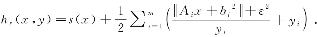
whereXis a given convex set,Aiandbiare given matrices and vectors, ands(x) is some continuously differentiable convex function. This problem was considered and solved in [2] by applying the IRLS method to its smoothed approximation problem:

(15)

or equivalently, by applying the original AM method to an auxiliary problem

(16)

where for a given setZthe indicator functionδ(x,Z) is defined by

(17)

(18a)

(18b)

In [2], the author first established the sublinear rate of convergence for the AM method and hence the same convergence result for the IRLS method follows. However, in many cases the subproblem of updatingxkis very hard to solve and even prohibitive for large-scale problems. It is just this drawback motivating us to propose AM-variant-I. Now, applying AM-variant-I and with some simple calculation, we at once obtain a linearized scheme of the IRLS method, that is

(19a)

(19b)

wherePXis the projection operator ontoX. IfPXcan be easily computed, then the linearized scheme becomes very simple. In addition, its sublinear rate of convergence can be guaranteed by Theorem 1. Nevertheless, we would like to point out that the scheme (34) can also be obtained by applying the proximal forward-backward (PFB) method [6] to the following problem

(20)

(21)

whereA∈Rm×nand the proximal operators offandgcan be easily computed. In [2], the author applied the AM method to its auxiliary problem

(22)

and obtained the following scheme:

(23a)

(23b)

Because the entries of vectorxare coupled byAx, the updating ofxkis usually very hard for large-scale problems. AM-variant-I fixes this problem and generates the following simple scheme:

(24a)

(24b)

5 Discussion

In this paper, we discussed a group of variants of the AM method and derived the sublinear rates of convergence under very minimal assumptions. Although we restricted our attention onto convex optimization problems, these variants for nonconvex optimization problems might obtain computational advantages over the AM method as well. Because our theory is limited to convex optimization, the convergence of AM-variant-I and AM-variant-II for general cases is unclear at present. In future pursuit, we will analyze the convergence of AM-variant-I and AM-variant-II under the nonconvex setting.

6 Proof details

6.1 Proof of Theorem 1

(25a)

(25b)

On the other hand, sinceyk+1minimizes the objectiveH(xk+1,y)+g(y), it holds that

(26)

By summing up the above two inequalities, we obtain

(27)

Step 2: prove the property (b). By Lemma 1, we have that

(28)

By the convexity ofH(z), it follows thatH(zk)-H(z*)≤∇H(zk),zk-z*. Thus,

(29)

f(x*)≥f(xk+1)+ckxk-xk+1,x*-xk+1+<∇xH(xk,yk),xk+1-x*>

(30)

and

g(y*)≥g(yk)+<∇yH(xk,yk),yk-y*>.

(31)

By summing up the above two inequalities, we obtain

(32)

Combining inequalities (48) and (51) and noticingγ>1, we have that

(33)

From inequalities (25b) and (26), it follows that

(34)

(35)

6.2 Proof of Theorem 2

Step 1: prove the property (a). Sincexk+1andyk+1are the minimizers to the subproblems in (6) respectively, we get that

(36)

and

(37)

By summing up the above two inequalities, we obtain

(38)

By the convexity ofH(z), it follows that

H(zk)-H(zk+1)≥<∇H(zk+1),zk-zk+1>.

(39)

By summing up the above two inequalities, we get

(40)

By Assumption 7, it holds that

(41)

(42)

Now, combining inequalities (40), (41) and (42), we finally get that

(43)

Step 2: prove the property (b). By Assumption 7 and Lemma 1, we have

(44)

The convexity ofH(z) impliesH(zk)-H(z*)≤<∇H(zk),zk-z*>. Thus, we get

(45)

Applying Lemma 2 to (10), we obtain that

f(x*)≥f(xk+1)+ck+<∇xH(xk,yk),xk+1-x*>

(46)

and

g(y*)≥g(yk+1)+dk+<∇yH(xk,yk),yk+1-y*>.

(47)

By summing the above two inequalities, we get

K(z*)≥K(zk+1)+ck+dk
+<∇H(zk),zk+1-z*>.

(48)

Combining inequalities (45) and (48), we have

(49)

(50)

(51)

6.3 Proof of Theorem 3

Step 1: prove the property (a). Sincexk+1andyk+1are the minimizers to the subproblems in (18) respectively, we get that

(52)

and

(53)

By summing up the above two inequalities, we obtain

(54)

Sinceρ1=inf{ck,dk:k∈N}>0, we have

(55)

Thus, we finally get

(56)

Step 2: prove the property (b). Applying Lemma 2 to (18), we obtain that

f(x*)≥f(xk+1)+ck+<∇xH(xk+1,yk),xk+1-x*>

(57)

and

g(y*)≥g(yk+1)+dk+<∇yH(xk+1,yk+1),yk+1-y*>.

(58)

By summing up the above two inequalities and letting

we obtain

(59)

By the convexity ofH(z), it follows that

H(zk+1)-H(z*)≤<∇H(zk+1),zk+1-z*>.

(60)

Thus, combining (59) and (60) yields

By Assumptions 6 and 8, we deduce that

<∇xH(xk+1,yk+1)-∇xH(xk+1,yk),xk+1-x*>

(61a)

(61b)

(61c)

By the Cauchy-Schwartz inequality and the notationρ2=sup{ck,dk:k∈N}, we have

(62)

(63a)

(63b)

This completes the proof.

6.4 Proof of Theorem 4

Step 1: prove the property (a). The following proof appeared in [5]. For completion, we include it here. Applying Lemma 3 to the scheme (12), we derive that

(64a)

(64b)

and

(65a)

(65b)

By summing up the above two inequalities, we obtain that

(66)

By Assumption 8, we finally get that

(67)

Step 2: prove the property (b). Applying Lemma 2 to (12), we obtain that

f(x*)≥f(xk+1)+ck+<∇xH(xk,yk),xk+1-x*>

(68)

and

g(y*)≥g(yk+1)+dk+<∇yH(xk+1,yk),yk+1-y*>.

(69)

By summing up the above two inequalities and letting

we obtain that

(70)

By Assumption 4 and Lemma 1, we have that

(71a)

(71b)

By Assumption 3 and Lemma 1 and the convexity ofH(z), we derive that

(72a)

(72b)

By summing up inequalities (71) and (72), we get

(73)

Together with (70) and utilizing Assumption 5 and the factγ>1, we derive that

(74a)

(74b)

(74c)

(74d)

(74e)