Wentao Tang,Prodromos Daoutidis

Department of Chemical Engineering and Materials Science,University of Minnesota,Minneapolis,MN 55455,USA

ABSTRACT Large-scale and complex process systems are essentially interconnected networks.The automated operation of such process networks requires the solution of control and optimization problems in a distributed manner.In this approach,the network is decomposed into several subsystems,each of which is under the supervision of a corresponding computing agent(controller,optimizer).The agents coordinate their control and optimization decisions based on information communication among them.In recent years,algorithms and methods for distributed control and optimization are undergoing rapid development.In this paper,we provide a comprehensive,up-to-date review with perspectives and discussions on possible future directions.

Keywords:Distributed control Distributed optimization Process networks Decision making

1.Introduction

Large-scale and complex systems have become prevalent in chemical and energy industries.Such systems arise from the integration of process units and plants as a result of sustainability motivations,specifically,economic efficiency,energy recycle,and carbon and water footprint reduction[1,2].Examples of such complex systems include chemical plants with recycles [3,4],crude oil refineries [5],smart grids and microgrids [6],integrated heating,ventilation and air conditioning (HVAC) systems [7],and supply chains [8,9].

Process control and optimization technologies are crucial to the implementation of such sustainable solutions in the chemical,energy and other relevant industry sectors.However,control and optimization become difficult for these large-scale and complex systems due to the size of their models and the existence of phenomena that emerge at a network level,such as multi-time-scale dynamics [10],multi-level uncertainties [11],and propagation of disturbances[12].These challenges to the control and optimization of process networks call for theoretical efforts to deal with each individual phenomenon,and a computational architecture for control and optimization that accounts for their networked nature.

A promising approach to this end is to make the control and optimization decisions in a distributed manner.Specifically,a distributed architecture of control and optimization has the following meaning:

· The entire process system,as a network,is decomposed into several constituent subsystems.

· A computing agent (controller,optimizer) is associated with each subsystem and is responsible for making the decision in the corresponding subsystem.

· Some information is exchanged between the agents to coordinate their decisions towards the control or optimization objective of the entire network.

A distributed architecture is different from a centralized one,in the sense that the decisions are made by multiple agents rather than a single agent.Compared to its centralized counterpart,distributed control and optimization are more scalable and parallelizable,and hence can be more efficient computationally.Moreover,a distributed architecture is flexible to the entering,exiting,and changes of subsystems(“plug-and-play”property[13]),and can be also combined with distributed fault detection for a fault-tolerant control architecture[14,15].It is also different from a decentralized architecture (which appears in traditional process control) due to the existence of some coordination mechanism,which generally enables the agents to account for other subsystems and arrive at desirable or optimal decisions for the overall network.

This paper provides a comprehensive and up-to-date review of distributed control and optimization.We aim to present the fundamental ideas and guide the readers through the most significant developments in recent years.The paper is organized as follows.We first introduce in Section 2 the preliminary concepts for the distributed architecture of control and optimization.Two major issues in developing a distributed control or optimization scheme,namely the methods of decomposing the network into subsystems,and the methods of performing optimization based on a network decomposition,are reviewed in Section 3 and Section 4,respectively.A case study on a reactor-separator process network is shown in Section 5.We discuss some important future directions in Section 6.Conclusions are made in Section 7.

2.Distributed Control and Optimization on Networks

2.1.Control and optimization

In the operations of process systems,many decisions need to be made.Decision making problems are organized in a hierarchy which contains the following problems on different time and space scales [8,16]:

· Control — input variables (flow rates,heat exchange rates,etc.)are manipulated to stabilize the system states (temperature,pressure,etc.) at their setpoints or track reference trajectories in a time scale of minutes to hours.

· Real-time optimization—the setpoints or reference trajectories are determined so as to optimize the economic performance under current market conditions.Such decisions are made in the time scale of hours to days.

· Scheduling — the sequence,timing and processing quantities are determined for the production equipment to meet the production goals over a time scale of days to weeks.

· Planning — high-level decisions such as production levels and product inventories are determined based on demand and marketing forecasts over weeks to months.

· Supply chain management — decisions on the material,information and financial flows between different business entities,including suppliers,producers,distributors and retailers,are made for enterprise-wide optimization.

An illustration of such a hierarchy is shown in Fig.1.Traditionally,these problems are solved separately,where any lower layer decisions are made under given higher layer decisions.The integration of these decision making problems,which is necessary especially under dynamic market conditions,is an area of active recent research [17-20].

The aforementioned operational decisions are typically determined through the solution of the corresponding optimization problems.Such optimization formulations are well established in the literature of process systems engineering[21,22]by specifying the relevant variables,defining the objective function,and modeling the process system as the constraints involving these optimization variables.For example,using a state-task or resource-task network to model the process units and materials,mixed-integer linear and nonlinear programming(MILP,MINLP)formulations can be derived for scheduling problems(see e.g.[23-25]for reviews).Optimization is also applied to the control decisions in the form of model predictive control(MPC)[26,27].If the objective function is an economic one,the control strategy is called economic model predictive control(EMPC) [28,29].In these approaches,suppose that we have the dynamical model of a process system:

where x(t) and u(t) are the vectors of states and control inputs at time t,respectively,and f is a vector-valued function.At any time t,the inputs are determined by solving the following optimal control problem involving the inputsand predicted statesin a future time horizon τ ∈[t,t+T]:

Fig.1.The hierarchy of decision making in process systems operations.

Here the objective function is the integral of φ,which represents a cost or performance loss,and a terminal cost ψ.The constraints contain the system dynamics,and possibly additional operational constraints such as input boundsThe problem(2)can be solved with different approaches through discretization of u(τ)and x(τ)in[t,t+T].Then the control decisions at the current time t are determined as u（t ）=.

The centralized framework of decision making is represented in Fig.2(a).The agent is the decision maker,namely a controller(optimizer),which receives the information required for decision making from the system and sends the decisions back to the system.For example,in control problems,the agent (controller) receives the state variables x(t) from the sensors,determines the control inputs u(t) (depending on x(t) as a parameter,thus also denoted by u(x(t))) and sends them to the actuators to execute the control signals.The agent and system thus compose a closed-loop systemevolving with time.

Fig.2.Decision making in (a) centralized and (b) distributed architectures.

2.2.Distributed control and optimization

For large-scale and complex systems,centralized decision making using the monolithic system model is usually computationally difficult,since in most cases,the associated optimization problems are intrinsically nonscalable as the problem size grows.Also,due to the dependence of all the decisions on all the system information,such a centralized control or optimization scheme is inflexible to any changes or faults in the plant,actuators or sensors.To avoid such limitations,distributed computing offers a more scalable,parallelizable and flexible paradigm for decision making [30].In recent extensive research works,this has been addressed in the contexts of distributed linear feedback control [31,32],distributed dissipativity-based control [33,34],distributed nonlinear model predictive control [35-37],distributed power scheduling [38,39]and economic real-time optimization [40,41].

The architecture for such a decision making is shown in Fig.2(b).The entire network is decomposed into constituent subsystems with interactions between them,e.g.,a tightly integrated chemical plant is partitioned into groups of process units.An agent is associated with each subsystem.The agents receive information from the corresponding subsystems,generate decisions,and transmit the determined decisions back to the subsystems.Due to the existence of interactions among the subsystems,it is insufficient to make decisions with separate agents,i.e.to use a decentralized architecture where each agent makes part of the decisions on its own.Instead,communication channels need to be establishedamong the interacting agents,through which the agents share certain information such as their local measurements and decisions.In this way,the mutual influences between the subsystems can be accounted for by the agents,and hence the computation of all the agents can be coordinated to meet an objective for the entire system.

In the context of distributed control and optimization,we consider the following aspects to be important:

(a) The development of network decomposition methods and the studies on the relation between decompositions and the resulting performance help to specify an optimal decomposition for distributed control and optimization.

(b) The development of distributed optimization algorithms and the studies on their convergence properties and numerical performance help to implement a more computationally efficient decision-making scheme.

(c) The non-ideality of communications will induce constraints on the control and optimization performances.The methods of analyzing and accommodating these communication network-induced issues help to improve the feasibility and flexibility of distributed decision.

Among the above three aspects,the communication issues have been addressed in a less unifying and non-universally applicable way.We will review the network decomposition methods and distributed optimization methods in the following two sections,respectively,and communication issues in the following subsection.

2.3.Issues with communication network

In distributed control and optimization,the communication among the agents as well as the communication between the agents and the system,are enabled by a communication network technology,including field-bus,controller-area network (CAN),Ethernet and Internet [42,43].However,any communication network has a limited capacity,which results in several so-called network-induced constraints [44].The influence of such network-induced constraints on the distributed optimization or closed-loop performance needs to be analyzed or accommodated.

In the context of distributed optimization using communication networks,the following problems have been studied:

· When the agents have different processing speeds,asynchronous iterations can be computationally more efficient than the ideally synchronized iterations.Asynchronous algorithms of distributed optimization have recently been developed [45,46].

· Due to the quantization of signals transmitted between the agents,distributed optimization algorithms with inexact communication have been developed [47,48],and the conditions on quantization for maintaining convergence properties have been studied [49].

· Event-triggered communication can reduce the communication cost,where the agents maintain estimations of the decisions of its neighboring agents,and the communication is triggered when this estimation deviates from the true values beyond a threshold [50,51].Such methods have been applied to optimal power flow problems [52,53].

· Another approach to reduce the communication requirement is to develop communication-efficient distributed optimization algorithms[54]with a tradeoff between exact steps with communication and inexact steps with only local information[55-57].

The effect and accommodation of network-induced constraints on the closed-loop system have been extensively studied in the context of networked control systems,assuming that an explicit form of control law is given,or that the system and the controller are prescribed to be linear.Typically,these constraints are regarded as uncertainties or combined with the original dynamics into a stochastic switched system or hybrid discrete-continuous system.Based on such models,the existence and synthesis of Lyapunov functions are used for stability analysis.These networkinduced constraints include:

· Time delay on the network.Time delays were treated as uncertainties in a robust stability framework[58]or in the context of switched systems[59].Delays can also be considered in the stability analysis of model predictive control [60-62].

· Missing and time reversal of transmitted information,i.e.package dropout and disorder.These can be accommodated by robust controller design[63],adaptive control[64,65],or transmitted data checking [66].Simultaneous package dropout and time delay were considered in [67].

· Information is sampled only on specific transmission time instants.The modeling of system behavior with discrete transmission times was addressed in [68],and together with time delay and package loss in [69].

· Competition of multiple nodes accessing the communication network.When such a competition exists,a time scheduling protocol,such as a round-robin or try-once-discard protocol,is needed[70]and has been analyzed together with other issues[71].

· Errors resulting from the signal quantization.The simultaneous presence of quantization errors along with the previous issues are considered in [72,73].A hybrid system model in the presence of all the previous issues is proposed in [74].

Event-triggered control (ETC) provides a possibility to largely relieve the communication burden for networked control,which has become the focus of more recent studies[75-77].The key idea underlying ETC is to make control decisions without information from the sensors using an approximate model and restore the communication only if such decision leads to a significant error.Eventtriggered model predictive control(ET-MPC)for linear systems has been addressed in [78,79].

The aforementioned issues associated with the communication network are illustrated in Fig.3.In a general setting of distributed control and optimization,we will have a closed-loop system comprising of a non-ideal communication network,distributed optimization-based agents and interacting subsystems with nonlinear dynamics.To this end,a generic framework of analyzing and accommodating the network-induced issues,or eventtriggered decision making,remains to be explored.

Fig.3.Illustration of communication network-induced issues.

3.Methods of Network Decomposition

3.1.Graph-theoretic algorithms

Graph theory is an important mathematical tool for interaction analysis and system decomposition,which dates back to the fundamental problem of solving large-scale linear equation systems Ax=b without inverting the entire large coefficient matrix (see e.g.[81]for an early review).Graphs comprise of nodes and edges connecting the nodes,which can represent the components of a system and their interactions,respectively.Depending on the systems and problems of interest,different types of graphs can be used:directed and undirected(whether each edge has a direction),weighted and unweighted (whether each edge has a weight),unipartite and bipartite(whether the nodes are homogeneous,or classified into two categories so that the edges only exist between nodes of different categories);see e.g.[82].

A major approach to the graph theoretic-based decomposition,widely used in traditional decentralized control,is the identification of a hierarchy of subgraphs [83],such as strongly connected components (the subgraphs in which a path exists from v1to v2and a path exists from v2to v1for any two nodes v1,v2in the subgraph)[84]or structurally controllable subsystems[85].With such an exposure of the interaction pattern underlying the graph,a decomposition is generated to facilitate the decentralized control design.For example,Fig.4 shows a directed graph representation[86]of a control system=f（x，u）,y=h(x),where the nodes u,x,y represent input,state,output variables,respectively,and the directed edges indicate the causal relations between the variables.After the decomposition according to the algorithm of[85],a hierarchical interaction pattern is exhibited between the subsystems(I →II,I →III,II →III).However,these methods are only applicable if a directed graph representation of the system is used and there exists a hierarchical structure.

Fig.4.Graph decomposition of a control system into subsystems with hierarchical interaction pattern.

More generally,the network needs to be decomposed with a partition,i.e.some edges need to be cut down to disconnect the graph[87].The graph partitioning problem can be directly formulated as an integer optimization problem (see e.g.[88]),which,however,is usually computationally difficult.The most prevalent approach is to consider recursive bisections,where each bisection is determined using a spectral algorithm with a heuristic fine-tuning procedure that seeks to minimize the cut edges(see e.g.[89]).We note that for distributed computing,it is desirable to impose balanced computational loads on the agents,which requires the sizes of the resulting subsystems to be uniform.To this end,approximately equal-size partitioning algorithms have also been proposed in[90]and applied to the Barcelona water network.We note that graph partitioning algorithms have wide applications in computer science and very-large-scale integration(VLSI)technology.For recent developments in graph partitioning,the readers are referred to [91].

3.2.Clustering algorithms

Clustering algorithms are widely used in the areas of data mining and machine learning.By defining a distance metric between the data points,clusters (groups) of mutually close points are formed,which helps to reveal the underlying organization of the dataset [92,93].Hierarchical clustering is a major class of clustering algorithms [94],which generates a dendrogram of clusterings through successive agglomeration or division.

Hierarchical clustering of input and output variables was used to decompose control systems based on relative degrees [95]as input-output distance measures.In [96],the inputs and outputs are first paired with minimized total relative degrees,and the input-output pairs are then agglomeratively clustered based on their mutual distances.An improved implementation of this algorithm was proposed in [97],and an extension to control systems with both ordinary and partial differential equations was addressed in [98].In [99],divisive hierarchical clustering method is used,where the dendrogram is generated through recursive bisections,and each bisection is determined by properly defined quality indices.

For illustration,Fig.5 illustrates the pairing of input and output variables and the dendrogram obtained by hierarchical clustering of the input-output pairs for a solid oxide fuel cell system [96].We note that the hierarchical clustering algorithm usually allows multiple solutions without determining an optimal decomposition.

Fig.5.Pairing and hierarchical clustering of inputs and outputs generated for a solid oxide fuel cell system.u and y represent inputs and outputs,respectively,and P1,...,P5 are input-output pairs.d is an input-output distance measure.

3.3.Community detection algorithms

Different from the approaches in the previous subsections,community detection as a major area of study in network science[100],provides a new perspective and efficient tools for decomposing large and complex networks.

Network science focuses on the macroscopic,statistical and coarse-grained properties of networks.By investigating examples of biological and social networks[101],it has been recognized that in many networks,the nodes can be assigned to several groups,called communities,such that the interactions inside the communities are stronger(denser)than the interactions between communities with a statistical significance.The mainstream community detection algorithms,including the well-known Louvain algorithm(fast unfolding algorithm) [102],belong to the type of modularity maximization [103,104],where a quantitative index called modularity is defined for any grouping of the nodes,and the grouping with approximately maximum modularity is found.

Not far from Smyrna, where the merchant drives his loadedcamels, proudly arching their long necks as they journey beneath thelofty pines over holy ground, I saw a hedge of roses

For example,the modularity-based community detection algorithm for unipartite undirected networks[103]is described as follows.Suppose the network is represented by an n×n adjacency matrix A=[aij]where aij=1 if there is an edge between node i and node j,and aij=0 if nodes i and j are non-adjacent,i,j=1,...,n.Let kibe the degree of node i,i.e.the number of edges incident to node i,and 2m the total number of edges (with each edge double counted):

The modularity of any grouping of the nodes is defined as

where Ciis the community affiliation of node i,and δ(Ci,Cj) is 1 if Ci=Cjand 0 otherwise.In the parentheses,aij/2m is the fraction of edges lying between nodes i and j;ki/2m is the fraction of edges incident to i,and thus kikj/4m2is the expected fraction of edges lying between i and j when the edges in the network are randomly redistributed while keeping the degrees of all the nodes constant.Therefore the difference between aij/2m and kikj/4m2captures the statistical significance of the connectedness of nodes i and j.Q defined in Eq.(4)is the intra-community sum of such differences,and characterizes the statistical significance of the existence of communities as specified by(C1,...,Cn).The modularity-based community detection is thus an (approximate) maximization of Q over(C1,...,Cn).

Many other efficient algorithms have also been developed for detecting the community structures in networks (see [105]for a review),including the following representative ones.In label propagation (LPA) [106]and speaker-listener LPA (SLPA) algorithms[107],the nodes hold labels which keep being propagated between the adjacent nodes,and the converged labels are considered as the community affiliations.In Infomap [108],random walks are associated with the network to proxy the information flows on it,based on which the optimal information compression reveals the community structures.Stochastic block model (SBM) methods,which consider the community affiliations as latent labels of the nodes and infer these labels from the network information,have been a research focus more recently [109,110].

By decomposing a network into its communities,one can determine subsystems with strong intra-subsystem interactions and weak inter-subsystem interactions.Such a decomposition optimally concentrates the interactions inside the subsystems in the sense of statistical significance,and thus allows a distributed control or optimization architecture with minimal compromise in performance.

For decomposition of control systems,several network representations have been developed [111-113].Specifically,

· in [111],a directed graph representation called system digraph(see also e.g.[86]),is used to capture the structure of the interactions between input,state and output variables;

· in [112],the edges in the directed graph are weighted using sensitivities (coefficients in the linearized system,see also e.g.[114]),which capture the short-time dynamic response intensities,and a bipartite graph of inputs and outputs is constructed based on shortest path search in the directed graph;

· in [113],the edges in the input-output bipartite graph are weighted based on the relative time-averaged gain array,which is a measure of input-output interactions on a finite time scale(which typically matches the closed-loop time constant).

Based on the network representations,suitable community detection algorithms are applied correspondingly to generate the network decomposition for distributed control.As an illustration,Fig.6 shows the community-based decomposition of a vinyl acetate monomer plant,which involves 26 manipulated inputs,43 measured outputs,and 246 state variables (the detailed model is given in [115]).

Fig.6.Decomposition of vinyl acetate monomer plant(upper)based on community detection (lower).

For decomposition of optimization problems,community detection has also been proposed as a powerful method,and is currently undergoing active research.In[116],a unipartite graph representation of optimization problems was proposed and its decomposition by community detection was used to solve design optimization problems.In [117],a variable-constraint bipartite network and unipartite network representations of optimization problems were proposed,and the benefit of community detection-based decompositions was demonstrated with an artificial convex problem and an optimal control problem solved using different distributed optimization algorithms.In [118],some mixed-integer nonlinear programming problems that are difficult to tackle with current solvers were investigated,and it was found that the decomposition by community detection helps to shrink the duality gap with tighter upper or lower bounds.

4.Methods of Decomposition-based Optimization

In the previous section we have presented methods of network decomposition.Once a decomposition is determined for the process,one can solve large-scale optimization problems by employing distributed optimization algorithms,which prescribe how the distributed agents update their decisions and how the information is transferred among the agents.In this section,we introduce the basics of the two major classes of formulations and algorithms of performing distributed optimization,namely block coordinate descent (BCD) algorithms and Lagrangian/augmented Lagrangian algorithms.We also review recent developments in optimization algorithms and software implementations in view of their importance in improving the computational efficiency of distributed optimization.

4.1.Block coordinate descent (BCD) algorithms

We consider optimization problems where the objective function involves N groups of decision variables x1,...,xN,and the constraints are separable,i.e.the constraints only exist within each variable group:

The separability of the constraints indicates that the decisions can be made separately without causing infeasibility.On the other hand,the variables are entangled in the objective function f(otherwise the problem(5)is separated).Therefore,whenever a group of decision variables is updated,the information of other variables and the overall objective function is needed.In other words,each computing agent needs to communicate the other agents with their decision variables,and keep the knowledge of the entire system on how all the variables affect the objective function.

Under such an architecture,the problem (5) can be solved by a BCD algorithm [119],where each group of decision variables (i.e.block of coordinates)is optimized with all the other variables fixed at their current values,and the variable updates are iterated until convergence.Namely,

where:=stands for value assignment,and arg min is the argument of minimization,i.e.the minimizer.Fig.7 illustrates the distributed optimization architecture with a BCD algorithm to compute the decisions with 4 agents.

This architecture is widely employed in distributed model predictive control [120-122]and economic model predictive control[123,124].The control inputs in the prediction horizon for the N subsystems u1,...,uNare considered as the decision variables.The decision variables are subject to separable constraints(ui∈Ui,i=1,...,N),but entangled in the objective function J(u1,...,uN),which,for any given inputs u1,...,uN,is evaluated by extracting information from the corresponding trajectories predicted by an ordinary differential equation simulator (e.g.using the Runge-Kutta method).With such a formulation,each agent needs to communicate its decisions with all other agents and performs optimization based on the entire system model,i.e.

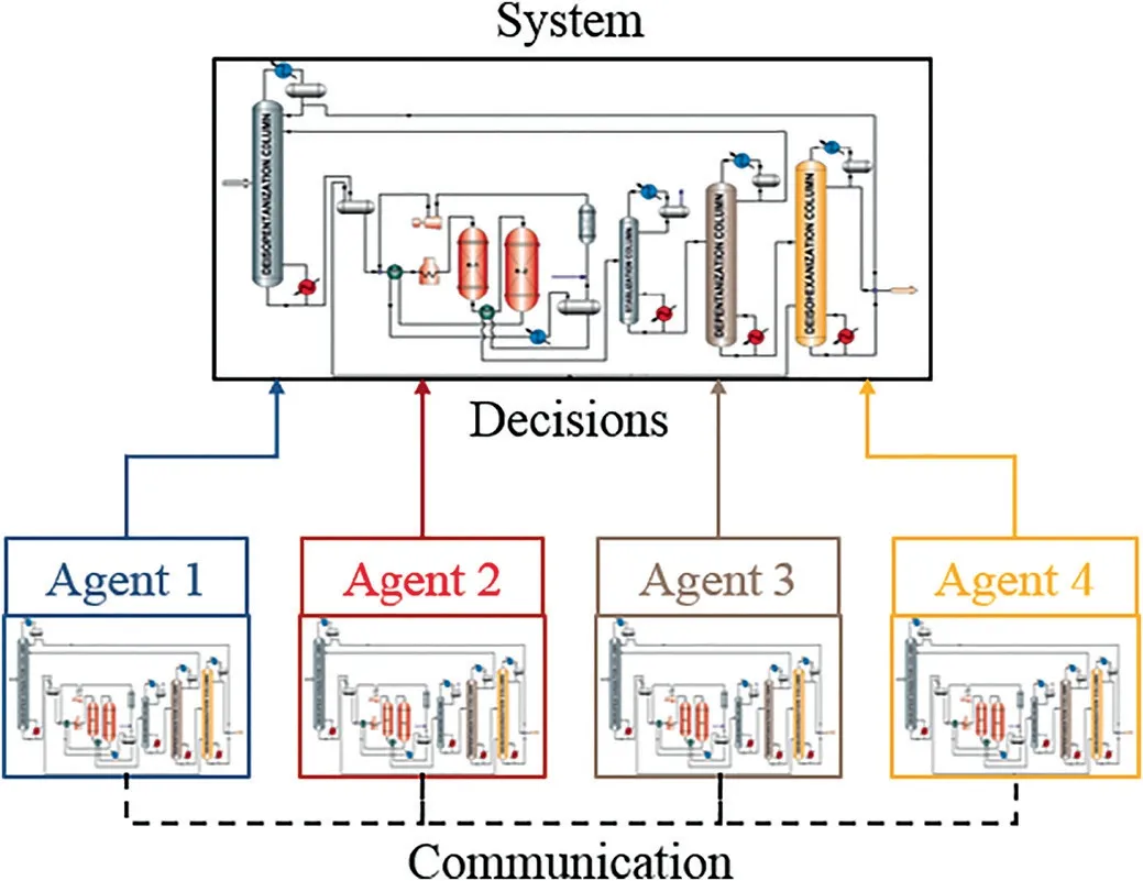
Fig.7.Distributed optimization architecture with BCD algorithm.The agents have the knowledge of the entire system,and communicate their decisions mutually.

The pristine algorithm in Eq.(6) has many variants.For example,instead of updating variables cyclically with fixed order,one may choose different selection rules of variable blocks,e.g.a randomized update rule [125],or parallelized update procedures[126];also,instead of directly minimizing f in each iteration,one may approximate f with a local linearization with proximal terms(e.g.quadratic regulation) [127].Under all these modifications,BCD-type algorithms can achieve a sublinear convergence rate[128,129].By incorporating Nesterov’s acceleration technique[130],computationally efficient implementations have been developed for convex problems [131,132].For nonconvex problems in general,BCD guarantees convergence under an assumption of the Kurdyka-Łojasiewicz property on the objective function f [133].

For distributed model predictive control,two major variants of BCD are typically considered,where the agents perform optimization in sequence and in parallel respectively[134].It was found for a benzene alkylation plant that the iteration number needed for BCD to solve each optimal control problem is small (convergent in about 15 iterations) [134].

4.2.Lagrangian and augmented Lagrangian algorithms

We consider optimization problems where the objective function can be separated into N terms (f(x)=f1(x1)+...+fN(xN)),each involving a group of decision variables,and linear equality constraints may exist between different variable groups in addition to the constraints within these groups:

Since the variable groups are separable in the objective function,i.e.a change in xionly influences the fi(xi) term of the objective function,each agent is allowed to keep the knowledge of only its subsystem model.On the other hand,due to the existence of linear constraints interconnecting different variable groups,any agent needs to communicate with its neighbors (the other agents whose corresponding subsystem contains variables interacting with the subsystem of this agent)to share the information of interacting variables.Fig.8 shows such an architecture.Compared to the previous architecture in Fig.7,this new distributed architecture is a truly localized and more flexible one,in the sense that only subsystem models and less communication burden between the agents are required.

With such an architecture,the problem (8) can be solved with the help of a Lagrangian decomposition [135].Define the dual variables λ associated with the linear constraints (which have an economic interpretation of shadow prices),and the Lagrangian

where the functions

Thus the problem (8) is reformulated as

The dual problem(11)is solved in a BCD-type algorithm,where the primal variables are minimized separately with the information of dual variables λ,followed by a dual update in its subgradient direction:

The step size α for dual update is typically chosen by Fisher’s rule [136],while other rules exist,such as the bundle method[137]and the surrogate subgradient method [138].

The performance of Lagrangian decomposition can be seriously affected by the nonconvexity of fiand Xi.Alternatively,one can adopt an augmented Lagrangian,where a quadratic penalty term for the linear constraints with ρ ＞0 is added to the Lagrangian to improve the convexity with respect to the primal variables [139]:

The so-called alternating direction method of multipliers(ADMM),as an augmented Lagrangian decomposition algorithm,is widely applied in machine learning [140]:

The step size parameter is chosen as γ ∈

The application of Lagrangian decomposition to scheduling and planning problems has been discussed in many relevant works[22,141,142].For distributed model predictive control,the application of Lagrangian decomposition [143-145]and ADMM[48,146,147]has also been proposed,for which the control decisions and the predicted states are taken as decision variables subject to constraints including the system dynamics.ADMM is also applied to other problems such as state estimation[148]and optimal power flow [149]on electricity grids.

Similar to BCD-type algorithms,variants of ADMM algorithms with parallelized[150]or randomized[151]variable updates have also been proposed,which are known to be sublinearly convergent for convex problems [152,153].To accelerate ADMM for convex problems,Nesterov’s technique has been proven to guarantee a quadratic convergence rate[154,155].Alternatively,for faster convergence,one may optimally fix the penalty parameter ρ [156]or use an adaptive penalty parameter throughout the iterations[157].For nonconvex problems,theoretical convergence under certain assumptions has also been discussed [158,159].However,the acceleration of nonconvex ADMM seems more difficult.Recently,we proposed an accelerated nonconvex ADMM algorithm where a discounted Nesterov’s acceleration scheme is incorporated into the parallelized ADMM [160].

4.3.Formulations,algorithms and software for optimization

In the previous subsections we have introduced BCD-type and Lagrangian-type distributed optimization algorithms and their corresponding communication architecture.Any distributed optimization algorithm is composed of iterated procedures of solving subproblems monolithically.It is desirable that these subproblems can be solved with high computational efficiency.To this end,we note that the following efforts are significant towards the efficient implementation of distributed optimization:

· Better formulations for problems of interest are being developed,which reduce the size or improve the convexity without losing the accuracy of the solution obtained.For example,to efficiently discretize continuous-time optimal control problems with small approximation error,collocation methods (pseudospectral methods)have been commonly adopted[161,162];to efficiently solve complex scheduling problems,reformulation methods[163]and approximation refinement techniques[164]have been proposed.The simplification of formulations using approximate or surrogate models seems especially crucial to integrated control and scheduling,which typically result in large-scale mixed integer dynamic optimization(MIDO)problems[165-167].

· Better optimization algorithms are also being developed to approach the optimum within fewer searching steps.For nonlinear programming problems (NLPs),e.g.for optimal control problems,the filtered line-search interior-point optimization(IPOPT) algorithm [168]usually exhibits a very fast convergence.Software packages have been developed to implement IPOPT as well as other interior-point optimization algorithms[169,170].With IPOPT,the parametric sensitivity of nonlinear programs can also be computed[171].Some recent works have focused on improving IPOPT by exploiting some special structures underlying the problem (e.g.optimal control problems typically have a tri-diagonal structure) [172,173].For mixed integer nonlinear programs (MINLPs),a number of global optimization solvers -BARON [174],ANTIGONE [175],LINDO API[176],SCIP [177],COUENNE [178]-have been developed and compared on libraries of benchmark problems.

· Better software platforms are being developed to automate the formulation(modeling)of optimization problems with less user effort and implement the algorithms with less computational time.For the optimization modeling,different from the traditionally used environments such as GAMS and AMPL which directly formulate the problems,algebraic modeling languages such as Pyomo [179]and JuMP [180]have been recently proposed.These are based on high-level programming languages(Python and Julia,respectively) and enable object-oriented modeling(e.g.[181]),i.e.automatic instead of manual formulation.For the efficient evaluation of derivatives during the solution of optimization problems,automatic differentiation packages(e.g.CasADi)have been developed and interfaced with modeling languages and solvers [182,183].

The roles of modeling language,automatic differentiation and solver in the solution of optimization problems are illustrated in Fig.9.So far,these efforts have been incorporated into toolboxes for model predictive control in a centralized architecture[184,185].For distributed control and optimization,open-source software packages are lacking.

Fig.9.The roles of modeling language,automatic differentiation and optimization solver.

5.Case Study on a Benchmark Process

In the works of our group,we have examined network decomposition and distributed optimization methods applied to the distributed MPC of a benchmark reactor-separator process[186,187].This system can be regarded as a minimal process network for distributed control and used for a demonstration of concept.For more complex processes,such as those appearing in oil refineries,indepth investigations need to be carried out and reported.

As illustrated in Fig.10,the process comprises two reactors,where first-order reactions A →B →C take place,and a separator from which the vapor phase is recycled and the liquid phase is withdrawn as product.The detailed dynamics and values of the parameters,steady states and inputs can be found in the aforementioned papers.The model contains 12 state variables,including holdup volumes(V1,V2,V3),and temperatures (T1,T2,T3) and concentrations (xA1,xA2,xA3,xB1,xB2,xB3),and 9 inputs,including flow rates (Ff1,Ff2,F1,F2,F3,FR) and heat exchange rates (Q1,Q2,Q3).From the 12 states,9 are considered as outputs (except for xA1,xA2,xA3).

Fig.10.Reactor-separator process.

5.1.Studies on network decomposition methods

For the reactor-separator process,we have considered the effect of network decomposition methods on the distributed model predictive control.Different network decompositions were generated based on respective decomposition methods,as summarized in Table 1.Specifically,

· Decomposition 1 is a centralized architecture with a single subsystem containing all inputs and outputs.

· Decomposition 2 is obtained by community detection based on relative time-averaged gain array (RTAGA) [113]that captures the finite-time interaction strengths between the variables.The RTAGA techniques tend to generate fine decompositions with a large number of subsystems.

· Decomposition 3 is obtained by community detection in a weighted directed graph representation that captures the short-time interaction strengths between the variables [112].

· Decomposition 4 is obtained by community detection in the unweighted directed graph representation that captures the structural interactions between the variables [111].

· Decomposition 5 is intuitively obtained based on the network topology (reactor 1+reactor 2+separator).The specific topology of the reactor-separator process makes it similar to decomposition 4.

Table 1 Decompositions obtained by different methods for the benchmark process

· Decomposition 6 is intuitively obtained considering mass and energy balances (feed and recycle flow rates affect concentrations;inventory flow rates affect holdup volumes,heat exchange rates affect temperature).

Distributed MPC was simulated for these decompositions for a tracking control task in 6 h [187],during which the setpoint changes every 2 h.The integrated squared error plus integrated control signals (ISE+ISC),namely the objective function in the optimal control problem of MPC,was used as a control performance index.A low performance index indicates good performance.By comparing the performance indices and computational times for the 6 decompositions,it was observed that

· Centralized MPC has a high computational burden compared to distributed MPC,and is hence not favorable.

· Among the community detection methods,the method of[111](decomposition 4)results in control performance comparable to the centralized MPC (7.2×103compared to 6.5×103),while largely reducing the computational time (2.6 min compared to 15.0 min).It also outcompetes the method of[112](decomposition 3).The method of [113](decomposition 2) has a deteriorated performance but a low computational cost due to a finer decomposition into 7 subsystems.

· The intuitive decomposition 6 is not favored,with a higher performance index and longer computational time than decomposition 4.Decomposition 5 has very close performance to decomposition 4,since the subsystem assignments of the variables are similar.

Therefore,we advocate community detection,especially the method of [111],as a beneficial tool to generate a high-quality decomposition for distributed control.

5.2.Studies on distributed optimization methods

We also studied distributed optimization methods for the reactor-separator benchmark process.In [187],the computational times of distributed MPC were compared using two different solvers — IPOPT and the traditional sequential quadratic programming (SQP).It was noted that IPOPT reduces the computational time approximately 60% compared to SQP for all the decompositions mentioned in the previous subsection.

Fig.11.Comparison of different ADMM algorithms.

When the agents only know the model of the corresponding subsystem instead of the whole plant,BCD cannot be used as a localized distributed optimization algorithm.In such a setting,we used the decomposition 4 in Table 1 and consider the tracking control of the benchmark process.3 ADMM algorithms were investigated,namely sequential (Gauss-Seidel),parallel (Jacobiproximal)and accelerated parallel(discounted Nesterov),depending on the way that the primal variables are updated[160].Under the ADMM algorithms,the closed-loop system is stabilized in 5 h.Fig.11 shows the comparison of 3 ADMM algorithms in terms of their performance indices,total ADMM iterations,and computational times (with an IPOPT solver).

· Among the ADMM algorithms,the accelerated parallel algorithm reduces the computational time up to 47% compared to the classical sequential algorithm.On the other hand,by using parallelization,the communication cost (number of iterations)inevitably increases.

· All ADMM algorithms lead to identical control trajectories (see[160]) with a stabilizing time of about 5 h and a performance index of 1.32×104.In this sense,distributed algorithms of the ADMM type are more robust than BCD.

· Both the control performance and computational efficiency of ADMM are deteriorated compared to BCD.The underlying reason is that when the agents only know the models of the local subsystems,it takes more iterations to coordinate the agents in ADMM.Although in ADMM,each optimization step based on local prediction is simpler than a BCD optimization step,due to the small size of the plant,this advantage of ADMM is not sufficient to overcome the demand for a large number of iterations for coordination in ADMM.

Therefore,it appears that BCD algorithms perform significantly better than ADMM if the system model is moderately complex and unchanged,while ADMM algorithms may be more suitable when the system model is large or frequently changing that BCD optimization steps based on the entire system information is intractable or unsuitable.

6.Future Directions

In the previous sections,we have reviewed up-to-date methods of distributed control and optimization.For the future development and industrial application of distributed control and optimization methods,in our opinion,the following directions are of importance:

· The communication network-induced issues need to be addressed in a more unifying framework that incorporates nonlinear systems and optimization-based,distributed agent decisions in a closed loop.

· The network decomposition and distributed optimization algorithms should be investigated for larger industrial systems,including those with units governed by partial differential equations.Comparison of different decomposition algorithms and different distributed optimization algorithms should be reported.Model reduction techniques may be necessary to make the distributed optimization algorithm real-time implementable for plant-wide systems.

· Algorithms lie at the heart of distributed control and optimization.The nonconvex nature of the control and optimization problems in process systems tends to increase the computational burden,and makes it more difficult to accelerate the algorithms than for convex problems.Moreover,for nonconvex problems,we are often required to find a global optimum rather than a local one,which gives rise to the problem of distributed global optimization.To this end,augmented Lagrangian-based global optimization algorithms[188]combined with global solvers such as ANTIGONE [175]or BARON[174],offer potential for distributed implementation.

· The modeling,decomposition and distributed control and optimization framework should be integrated into efficient software packages,so that the users do not have to run through all the details of these methods,as long as the necessary settings and information are provided.We notice the efforts to incorporate graph topology into distributed optimization software [189,190].It is also desirable to bridge this platform to existing commercial software for process design.

· Process monitoring,i.e.fault detection and diagnosis,is highly important to the process safety and product quality.Distributed process monitoring techniques have been proposed for both statistical[191,192]and model-based[193,194]approaches,where the monitors detect faults in the corresponding subsystems,and communicate to form the overall decision.For more advanced approaches e.g.using neural networks [195,196],distributed monitoring has not yet been addressed.Network decomposition methods for monitoring and their effects on the monitoring performance have only been studied recently[197].

· Data-driven control has been proposed as an alternative to the model-based control if an accurate control-oriented process model cannot be obtained [198].Data-driven control methods are mostly based on data-driven model identification(see[199]),or reinforcement learning (see [200]).So far,these methods are apparently applicable only to small-scale systems that are not highly nonlinear.Distributed algorithms for data-driven control and optimization of process networks are apparently in need.

7.Conclusions

Large-scale,complex process networks are prevalent in chemical and other industries due to economics and sustainability considerations.Distributed control and optimization have been identified as a crucial decision-making paradigm for the operation of such complex networks,and studied extensively in the recent years.In this review paper,we first introduced the basic concepts of distributed control and optimization.We reviewed two most important aspects of distributed control and optimization,namely the methods of determining a network decomposition,and the methods of performing optimization based on a network decomposition.A case study was used to illustrate these methods.We also briefly proposed some potential future directions.