Ze Zhao(赵泽)

School of Physical Sciences,University of Chinese Academy of Sciences,No.19A Yuquan Road,Beijing 100049,China CAS Key Laboratory of Theoretical Physics,Institute of Theoretical Physics,Chinese Academy of Sciences,Beijing 100190,China

Kavli Institute for Theoretical Physics China,Chinese Academy of Sciences,Beijing 100190,China

AbstractIn this work,we compare the impacts given by χ2statistics and Bayesian statistics.Bayesian statistics is a new statistical method proposed by[C.Ma,P.S.Corasaniti,and B.A.Bassett,arXiv:1603.08519[astro-ph.CO](2016)]recently,which gives a fully account for the standard-candle parameter dependence of the data covariance matrix.For this two statistical methods,we explore the possible redshift-dependence of stretch-luminosity parameter α and colorluminosity parameter β by using redshift tomography.By constraining the ΛCDM model,we check the consistency of cosmology-fit results given by the SN sample of each redshift bin.We also adopt the linear parametrization to explore the possible evolution of α and β and the deceleration parameter q(z)for CPL,JBP,BA and Wang models.We find that:(i)Using the full JLA data,at high redshift α has a trend of decreasing at more than 1.5σ confidence level(CL),and β has a significant trend of decreasing at more than 19σ CL.(ii)Compared with χ2statistics(constant α, β)and Bayesian statistics(constant α, β),Bayesian statistics(linear α and β)yields a larger best-fit value of fractional matter density Ωm0from JLA+CMB+GC data,which is much closer to slightly deviates from the best-fit result given by other cosmological observations.(iii)The figure of merit(FoM)given by JLA+CMB+GC data from Bayesian statistics is also larger than the FoM from χ2statistics,which indicates that former statistics has a better accuracy.(iv)q(z)given by both statistical methods favor an eternal cosmic acceleration at 1σ CL.

Key words:cosmology,dark energy,observations,cosmological parameters,supernova

1 Introduction

Type Ia supernova(SN Ia)is one type of supernova,which occurs from a terrific explosion of white dwarf star in binary systems.[1]SN Ia is named as the cosmological standard candle which can measure the history of the expansive universe.[2−3]For this reason,SN Ia has become one of the most effective observation to explore the essence of dark energy(DE).[4−12]Several supernova(SN)datasets have been released in recent years,such as “SNLS”,[13]“Union”,[14]“Constitution”,[15−16]“SDSS”,[17]“Union2”,[18]“SNLS3”,[19]and “Union2.1”.[20]“Joint Light-curve Analysis”(JLA)dataset is the latest SN sample,[21]which consists of 740 supernovae(SNe).And in the process of cosmology-fits,stretch-luminosity parameter α and colorluminosity parameter β are two important quantities of SN Ia which are treated as model-free parameters.[19−21]The aim of considering α and β is to reduce systematic uncertainties of SN Ia.

The possibility of the evolution of α and β with redshift z is one of the most important factors for controlling of the systematic uncertainties.So far,there is still no credible evidence in the past study for the evolution of α(z).On the other hand,the redshift-dependence of β has been supported by several SN datasets including Union2.1,[22]SNLS3,[23]and JLA.[24]Reference[23]states that β deviates from a constant at 6σ confidence level(CL)based on the SNLS3 samples.And by applying a linear β on studying various DE and modified gravity models,[25−28]the evolution of β has effects on parameter estimation,and assuming β as a time-varying form depress the tension between SN Ia and other cosmological observations.And also,Reference[29]found β at high redshift has a clear decreasing trend,at about 3.5σ CL.

Recently,Reference[30]have performed a Bayesian inference method for the JLA dataset using Bayesian graphical models to derive the full posterior distribution of fitting model parameters. Compared with the old χ2statistics,Bayesian statistics is a different statistical approach,which gives a statistically significant shift of the SN standard-candle corrections toward lower(absolute value).χ2fit does not fully propagate the parameter dependence of the covariance.In contrast,Bayesian inference gives a fully account for the standard-candle parameter dependence of the data covariance matrix.

In this work,we adopt Bayesian statistics on the analysis of redshift dependence of stretch and color by using redshift tomography.Redshift tomography method has been widely applied in the study of numerical cosmology.[31−33]The basic thought of this method is dividing the SN data into several redshift bins,and assuming α and β as piecewise constants in each bin.By using this method,we constrain Λ-cold-dark-matter(ΛCDM)model.And also,in each bin we check the reliability of cosmology-fit results.One of advantages by adopting the redshift tomography method is a reduction of statistical significance.Reference[30]adopt Bayesian statistical method on JLA data,and they only assume that α and β are constants.But we find from the results given by Bayesian statistics,α and β show a tendency of linear evolution with redshift z.Therefore,we further explore the possible evolution of α and β by taking linear parametrization of α and β.And we make a comparison between results of Bayesian statistics and χ2statistics.Furthermore,we consider the impacts of linear parametrization of α and β for CPL,JBP,BA and Wang models.For further study on modelindependent parameterizations,see Ref.[34].Figure of merit(FoM)is also calculated for these 4 models based on the combined JLA+BAO+GC data.And based on the JLA data only and the combined JLA+CMB+GC data,we also compare the values of fractional matter densityΩm0given by three cases:(i)χ2statistics with constant α and β.(ii)Bayesian statistics with constant α and β.(iii)Bayesian statistics with linear α and β.Moreover,to discuss the fate of the universe,we present the evolution of deceleration parameter q(z)for four models given by two statistical methods.

We state our method in Sec.2,show our results in Sec.3,and summarize in Sec.4.

2 Methodology

2.1 Theoretical Model

The comoving distance r(z)in a flat universe satisfiesis

where H0is the current Hubble constant and c is the speed of light.E(z)represents the reduced Hubble parameter given by

Here Ωr0, Ωm0and Ωde0are the present fractional densities of radiation,matter and dark energy,respectively.And X(z)is the DE density function,which is given by

where w represents the equation of state(EoS)of DE,that is one of determinative elements for the properties of DE.And specially,X=1,for the standard Λ-cold-darkmatter(ΛCDM)model.

To analyse the evolution of α(z)and β(z)for different models,we consider four important parametrization models:

(i)CPL model[35−36]has a dynamical EoS w(z)=w0+waz/(1+z),thus X(z)satisfies

(ii)JBP model[37−38]has a dynamical EoS w(z)=w0+waz/(1+z)2,thus X(z)satisfies

(iii) BA model[39]has a dynamical EoS w(z)=w0+waz(1+z)/[1+z2],thus X(z)satisfies

(iv) Wang model[40]has a dynamical EoS w(z)=w0(1−2z)/(1+z)+waz/(1+z)2,thus X(z)satisfies

Parameter w0describes the current value of EoS,and wareflects the evolution of EoS for each model.We also make use of the deceleration parameter q ≡ −/aH2to investigate the evolutionary behavior of cosmic acceleration(CA).

Figure of merit(FoM)was firstly proposed for the purpose of comparing different DE experiments.Making use of the CPL model,Dark Energy Task Force(DETF)constructs a quantitative expression of FoM,which is inversely proportional to the area enclosed by the 95%CL contour in the(w0,wa)plane:[41]

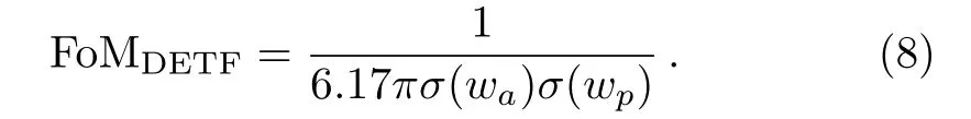
Here

Due to the relation σ(wa)σ(wp)=there is no need to calculate the conversion of wpfor the FoM.Evidently,largerFoM demonstrates better accuracy.In this paper,we apply the DETF version of FoM on CPL,JBP,BA and Wang models to compare χ2statistic with Bayesian statistic.

2.2 Observational Data

In this section,we firstly show the process of calculating the χ2function of JLA data for both χ2and Bayesian statistics.Then,we describe the details of the redshift tomography method.

In a flat universe,the distance modulus υthcan be calculated as

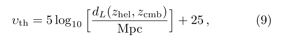
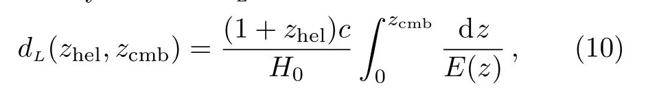
here zcmband zhelrepresent the cosmic microwave background(CMB)restframe and heliocentric redshifts of SN.The luminosity distance dLcan be written as

The observation of distance modulus υobscan be calculated by a empirical linear expression:

M⊙is the mass of sun.

The χ2of JLA data is calculated by the expression

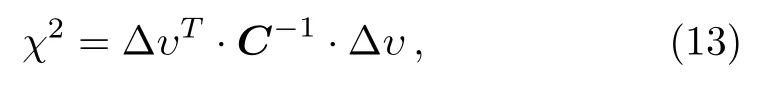
where∆υ ≡ υobs− υthis the data vector.C is the total covariance matrix,which is given by

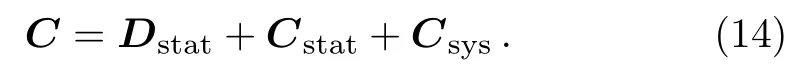
Dstatis the diagonal part of the statistical uncertainty,which is given by[21]

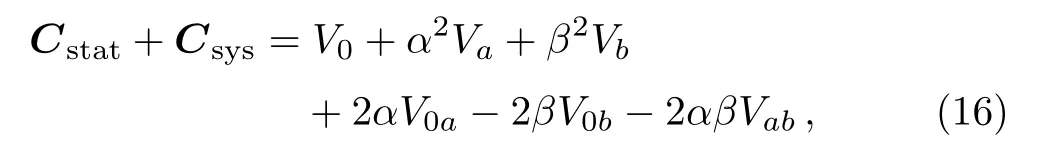
JLA group(http://supernovae.in2p3.fr/sdss−snls−jla/Re adMe.html)introduces matrices V0,Va,Vb,V0a,V0band Vab.And also Ref.[21]gives a detailed discussions towards to JLA SN sample.

For the methodology of Bayesian statistics,[30]the posterior probability is defined in Bayesian statistics as

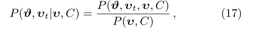
where υ is a distance modulus data vector with covariance matrix C,ϑ is a parameter vector for a specific theoretical model,distance modulus υt=ft(ϑ)is a deterministic function predicted by ϑ.The term P(ϑ,υt,υ,C)represents the joint probability distribution that can be written as:

by applying the chain rule of conditional probabilities.

Marginal probability is the integral of P(ϑ,υ1,υ,C)with respect to υt:

Z(υ,C)is a normalization constant defined by Z(υ,C)≡ P(υ,C)/P(C)=P(υ|C).Z(υ,C)is deterministic in model selection which is named by Bayesian evidence.Gaussian likelihood function L(ϑ;υ,C)can be written as

Take the logarithm of Eq.(19)and we have

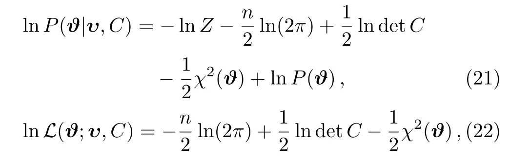
here

is the chi-square of the χ2statistics.Evidence variables C and υ in Eq.(19)is fixed by the dataset.After this consideration,Eq.(19)turns to a function of ϑ which is easily evaluated.For brevity,in this paper we will not make notational distinction of conditioning variables and their realized values in the equations.

The likelihood up to a normalization for χ2and Bayesian statistics can be calculated respectively as

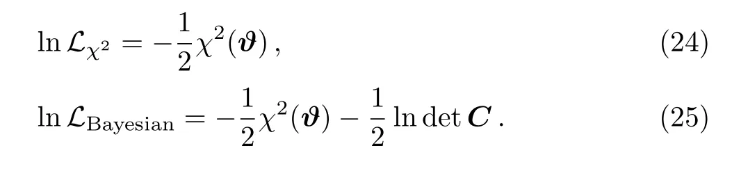
As pointed out in Ref.[30],compared with the Bayesian statistics,χ2approach shifts the standardization parameters away from the ideal standard candle case markedly.The standardization parameter given by χ2statistics also has larger values. As a matter of fact,lnL→lnLBayesian=lnL−(1/2)lndetC results in a distortion to the uniform prior of α and β to a certain extent.

It should be pointed out that,we marginalize the Hubble constant H0and the absolute B-band magnitude MBaccording during the process of calculating lnL.Readers can check the details of marginalized process and the code related to JLA likelihood from Ref.[21]As stated above,we aim at studying the possible evolution of α and β SN by adopting a model-independent method.Therefore we apply the redshift tomography method in this paper.The essential thought of redshift tomography is to split whole SN sample in several redshift bins.assuming that both α and β are are piecewise constants.By constraining the ΛCDM model,we check the consistency of cosmology-fit results given by the SN sample of each redshift bin.Furthermore,in order to make results insensitive to the details of redshift to mography,in this work we divide the JLA data sample at redshift region[0,1]uniformly into 3 bins,4 bins,and 5 bins.In each bin, α and β are assumed as piecewise constants in the fitting process.Based on different statistical methods including χ2and Bayesian statistics,We consider both α and β are constants and also adopting linear parametrization of α and β.We plot these related results together in order to compare the fitting results from different cases and data.In this work we use Markov Chain Monte Carlo(MCMC)methods to constrain parameters and analysis data by the assist of the CosmoMC package.For the details of this package,see Ref.[44]

3 Results

We compare the Bayesian and χ2statistics for the evolution of JLA luminosity parameters α and β.In Subsec.3.1,for the ΛCDM model,we revisit in the evolution of α and β using redshift tomography.In Subsec.3.2,we investigate the impacts of linear parametrization of α and β on the parameter estimation,and compare with the results of Subsec.3.1.And we further verify impacts of linear parametrization of α and β on different models including CPL,BA,JBP and Wang models.In Subsec.3.3,we also compare the values of fractional matter densityΩm0given by three cases:(i)χ2statistics with constant α and β.(ii)Bayesian statistics with constant α and β.(iii)Bayesian statistics with linear α and β.And results in this section are based on the JLA data only and the combined JLA+CMB+GC data.In Subsec.3.4,we further discuss the fate of universe by investigate the evolution of the deceleration parameter for both statistical methods by using JLA and JLA+CMB+GC data.

3.1 Revisit in the Evolution of α and β Using Redshift Tomography

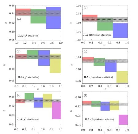
Fig.1(Color online)The 1σ confidence regions of stretch-luminosity parameter α(z)obtained from χ2statistics(a)–(c)and Bayesian statistics(d)–(f).for ΛCDM The results only consider the ΛCDM model,based on by using the full JLA samples at redshift zone[0,1].And 3 bins,4 bins,and 5 bins are shown in the upper,middle and lower panel.which are divided into 3 bins(upper panels),4 bins(middle panels),and 5 bins(lower panels).in which the absolute B-band magnitude MBare marginalized.The gray zone represents the 1σ region and the gray dashed line denotes the best-fit result given by the full JLA data.

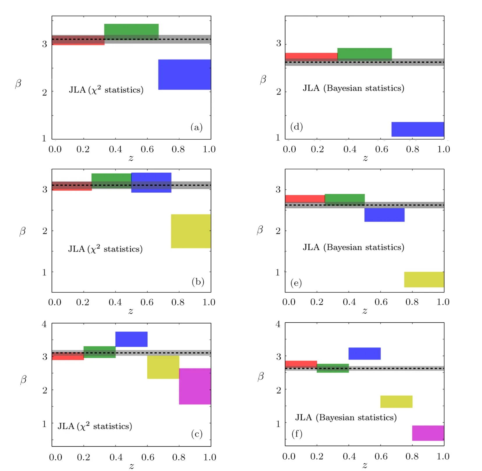
Fig.2(Color online)The 1σ confidence regions of stretch-luminosity parameter β(z)obtained from χ2statistics(a)–(c)and Bayesian statistics(d)–(f).for ΛCDM The results only consider the ΛCDM model by using the full JLA samples at redshift region[0,1].And 3 bins,4 bins and 5 bins are shown in the upper,middle,and lower panel.The gray zone represents the 1σ region and the gray dashed line denotes the best-fit result given by the full JLA data.

The major results in this section is comparing the evolution behaviors of JLA luminosity parameters α and β given by different statistical methods.i nd the evidence for the evolution of α with z,which is significantly different with previous value obtained from χ2statistics(see e.g.Ref.[29]).although it is consistent with a constant at low redshift.And meanwhile,Bayesian statistics reduce the error bar of α compare to χ2statistics.Specifically,α For the case of 3 bins,the 1σ upper frontier of α in the third bin deviates 1.5σ CL from the results obtained from the full JLA sample.For the case

In Fig.1,we present the 1σ confidence regions of stretch-luminosity parameter α obtained from χ2statistics(a)–(c)and Bayesian statistics(d)–(f).From left panels given by χ2statistics,apparently for the SN samples of 3 bin the 1σ regions of α consist with a constant.This conclusion is compliant with all the cases included 3 bins,4 bins and 5 bins,which is also in compliance with the results in other paper.[22−24,33]In contrast,for right panels given by Bayesian statistics,the results from SN samples of 3,4 and 5 bins have a significant trend of decreasing at high redshift.Therefore,by using Bayesian statistics,we f of 4 bins,the 1σ upper frontier of α in the forth bin deviates 3.8σ CL from the value obtained from full JLA sample.For the case of 5 bins,the 1σ upper frontier of α in the fifth bin deviates 4.1σ CL from the value obtained from the full JLA sample.(see Table 1).These deviations imply at high redshift,there is more than 1.5σ CL evidence for the decline of α.It should be pointed out this conclusion is not sensitive to the methods of redshift tomography.[29]

In Fig.2,we present the 1σ confidence regions of stretch-luminosity parameter β given by χ2statistics(a)–(c)and Bayesian statistics(d)–(f).For all left panels given by χ2statistics,there is a clear deviation from the results of full JLA sample at high redshift between the results obtained from SN samples of several bins Specifically,β has a significant trend of decline at high redshift.Although at low redshift,it consists with a constant.For all right panels given by Bayesian statistics,the decreasing tendency of β is more clear than the results given by χ2statistics.And meanwhile,Bayesian statistics reduce the error bar of β compare to χ2statistics.In details,There is a clear deviation at high redshift between the results given by SN samples of several bins from the results of full JLA sample.for the case of 3 bins,the 1σ upper frontier of β in the third bin deviates 19σ CL from the value obtained from the full JLA sample.For the case of 4 bins,the 1σ upper frontier of β in the forth bin deviates 24.4σ CL from the value obtained from the full JLA sample.For the case of 5 bins,the 1σ upper frontier of β in the fifth bin deviates 25.9σ CL from the value obtained from the full JLA sample.(see Table 1).These deviations imply at high redshift,there is more than 19σ CL evidence for the decline of β.And it is also not sensitive to the methods of redshift tomography.

For both the results of α and β,Bayesian statistics effectively reduce the error bar.This is because the χ2fit does not fully propagate the parameter dependence of the covariance which contributes with a lndetC term in the parameter posterior.From the decreasing tendency for the results given Bayesian statistics,it is necessary to consider the linear parametrization of α and β (see Subsec.3.2).

3.2 A Closer Investigation on the Impacts of Linear Parametrization for α and β

In this section, we consider introducing linear parametrization of α and β: α(z)= α0+ α1z and β(z)= β0+β1z.

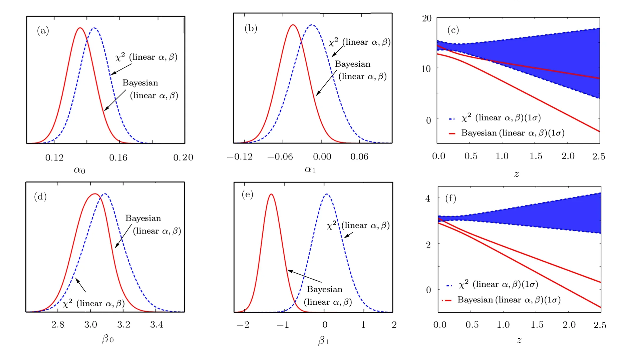
Fig.3 (Color online)The 1D marginalized probability distributions of α0, α1, β0, β1and the evolution of α(z),β(z)given by χ2statistics(blue dashed line)and Bayesian statistics(red solid line).Note that,we consider linear parametrization: α(z)= α0+α1z and β(z)= β0+ β1z for ΛCDM based on the full JLA sample.

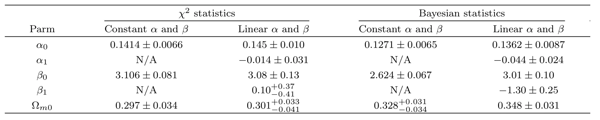
Table 1 Cosmology-fits results given by χ2statistics and Bayesian statistics for the ΛCDM model.For each statistical methods,we consider two cases:constant α and β;linear α and β.Both the best-fit result and the 1σ errors of parameters given by JLA data are listed in this table.

Table 1 presents the cosmology-fits results for the ΛCDM model obtained from χ2statistics with constant α, β, χ2statistics with linear α and β,Bayesian statistics with constant α, β and Bayesian statistics with linear α and β.From this table we can see that,the best-fit of the α1and β1from χ2statistics is much closer to zero than Bayesian results,which is also can be seen in Fig.3.For each statistical methods,taking linear parametrization of α and β leads to a larger Ωm0than the case of constant α and β.For the case of constant α, β and the case of linear α and β,adopting Bayesian statistics will also yield a larger Ωm0compared with χ2statistics.

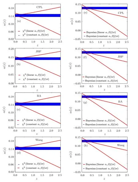
Fig.4(Color online)The evolution of β(z)for CPL,JBP,BA and Wang models obtained from χ2statistics(a)–(d)and Bayesian statistics(e)–(h).The results based on the full JLA samples at redshift region[0,1].The blue region denotes the 1σ confidence region of α for the case of constant α and β.The red solid line corresponds to the 1σ boundary for the case of linear α and β.

In Fig.3,we present the 1D marginalized probability distributions of α0,α1, β0, β1and the evolution of α(z),β(z)for the two statistical methods.Based on the full JLA sample,we consider the linear parametrization of α and β for the ΛCDM model.For χ2statistics,the center of the probability distributions for α1and β1is close to zero(see Table 1),which means,χ2statistics tends to the case that α and β are constant: α(z)= α0and β(z)= β0.As for the Bayesian statistics,the center of the probability distributions for both α1and β1show clear deviation from zero compared to results from χ2statistics.Which means,Bayesian statistics show much tendency of linear α and β with respect to redshift z than χ2statistics.And the evolution of α(z), β(z)Figs.3(e)and 3(f)also confirm the same evolutionary trend:the result of χ2statistics with linear α and β is consist with a constant;the result of Bayesian statistics with linear α and β show clear decreasing tendency which is not consist with a constant.

Figure 4 is the evolution of linear α(z)for CPL,JBP,BA and Wang models given by χ2statistics(a)–(d)and Bayesian statistics(e)–(h).Once adopting χ2statistics,the 1σ region of α for the case of constant α and β locates entirely in the 1σ region corresponds to linear α and β.For the Bayesian statistics,the 1σ region for the case of linear α and β show clear deviation from the region corresponds to the constant α and β at high redshift region.The decreasing tendency consists with the results of the ΛCDM model(lower panels of Figs.3).

Fig.5(Color online)The evolution of α(z)for CPL,JBP,BA and Wang models obtained from χ2statistics(a)–(d)and Bayesian statistics(e)–(h).The results based on the full JLA samples at redshift region[0,1].The blue region denotes the 1σ confidence region of α for the case of constant α and β.The red solid line corresponds to the 1σ boundary for the case of linear α and β.

In Fig.5,we plot the evolution of linear β(z)for CPL,JBP,BA,and Wang models obtained from χ2statistics(a)–(d)and Bayesian statistics(e)–(h).For χ2statistics,the 1σ region of β for the case of constant α and β locates entirely in the 1σ region corresponds to linear α and β.Based on the Bayesian statistics,the 1σ region for the case of linear α and β show clear deviation from the region corresponds to the constant α and β at high redshift region.Compared with the evolution of α in Figs.4(a)–4(d),the deviation of β is more evident and the overlapping region at low redshift is more tiny.The decreasing tendency consists with the results of the ΛCDM model Figs.3(e)and 3(f).

It should be mentioned that,for these two statistical methods,the results of α(z)and β(z)for CPL,JBP,BA and Wang models are very close,which is consistent with the model-independent methods we used.which means,the evolution of α(z)and β(z)are not depend on models.

3.3 Comparison of Ωm0Between χ2and Bayesian Statistics for CPL,JBP,BA and Wang Models

As shown in Fig.6,we present the 1D marginalized probability distributions of Ωm0for CPL,JBP,BA and Wang models given by different statistical methods.We apply χ2statistics with constant α, β (red solid line),Bayesian statistics with constant α,β (green dotted line)and Bayesian statistics with linear α,β (blue dashed line)based on full JLA data.For all 4 models,the best-fit ofΩm0given by Bayesian statistics with linear α,β is around 0.45,which is larger than the results given by the other case. Ωm0from χ2statistics with constant α, β is the minimum value among this three cases.This cosmological fitting is not ideal,because this results is based on the JLA data only,which is not capable to constrain the parameter Ωm0.Therefore,it is necessary to consider using combined observational data to constrain these parameters.

Fig.6(Color online)The 1D marginalized probability distributions of Ωm0for CPL,JBP,BA and Wang models given by different statistical methods.We apply χ2statistics with constant α, β (red solid line),Bayesian statistics with constant α,β (black dotted line)and Bayesian statistics with linear α,β (blue dashed line)based on full JLA data.

Based on the combined JLA+CMB+GC data,Fig.7 presents the 1D marginalized probability distributions ofΩm0obtained from different statistical methods.It should be pointed out that we use CMB data from Ref.[45]and other distance priors data from Refs.[46–48].And we use updated Galaxy Cluster(GC)data extracted from SDSS samples.[49]We apply χ2statistics with constant α,β (red solid line),Bayesian statistics with constant α, β(green dotted line)and Bayesian statistics with linear α,β(blue dashed line)on CPL,JBP,BA and Wang models.It is clear that Ωm0given by JLA+CMB+GC data is less than the values from JLA data on the whole.The best-fit of Ωm0given by Bayesian statistics with linear α,β is around 0.311(see Table 2),which is much closer to results of Ref.[45]than other two cases.Ωm0given by Bayesian statistics with linear α,β is less than the results from Bayesian statistics with linear α,β. Ωm0given by χ2statistics with constant α,β is still minimal among three cases.

Fig.7 (Color online)The 1D marginalized probability distributions of Ωm0by using χ2statistics with constant α, β(red solid line)and Bayesian statistics with linear α,β (blue dashed line).We consider the CPL,JBP,BA and Wang models respectively,based on the combined JLA+CMB+GC data.

Furthermore,we extend this comparison with more details.Table 2 presents the cosmology-fits results for the CPL,the JBP,the BA and the Wang models,obtained from χ2statistics with constant α, β,Bayesian statistics with constant α, β and Bayesian statistics with linear α,β. “χ2const” denotes χ2statistics with constant α and β.“Bayesian const” represents Bayesian statistics with constant α and β. “Bayesian linear”corresponds to Bayesian statistics with linear α and β.Both the best-fit result and the 1σ errors of these parameters,as well as the corresponding results of FoM are listed in this table.The combined JLA+CMB+GC data are used in the analysis.From Table 2,it is apparent to see that,for all the four DE models,the case of applying “Bayesian linear” will yield a larger Ωm0,compared with the cases of“χ2const” and“Bayesian const”.The comparison between these three cases is already shown in Fig.7.

Moreover,FoM given by Bayesian statistics is apparently larger than the values given by χ2statistics(constant α,β).For instance,for CPL model,FoM of Bayesian statistics is about two times Fom of χ2statistics.As we know,a larger value of FoM implies a better accuracy for constraining parameters.This means that we can obtain tighter DE constraints from Bayesian statistics.And it should be pointed out,since this conclusion is tenable for all these four DE parameterizations,our discussion is not sensitive to the specific model of DE.

3.4 An Extended Comparison of the Deceleration Parameter q(z)Given by JLA and JLA+CMB+GC

Figure 8 is the evolution of the deceleration parameter q(z)for CPL,JBP,BA and Wang model given by χ2and Bayesian statistics.

Fig.8 (Color online)The evolution of the deceleration parameter q(z)for CPL,JBP,BA and Wang model given by χ2and Bayesian statistics.The results based on the JLA only(a)–(d)and combined JLA+CMB+GC data(e)–(h).in which the absolute B-band magnitude MBare marginalized.The blue region denotes the 1σ region of q(z)for the case of χ2statistics with constant α and β.The red solid line corresponds to the 1σ boundary for the case of Bayesian statistics with linear α and β.

The results based on the JLA only(a)–(d)and combined JLA+CMB+GC data(e)–(h).From left panels,based on the JLA only,the 1σ region of q(z)for the case of Bayesian statistics(linear α,β)and χ2statistics(constant α,β)are partly overlapped.For four models given by two statistics,q(z)is consistent with an decreasing function at 1σ CL,which favor an eternal CA.Note that this results is also consistent with Ref.[50]From right panels,based on the combined JLA+CMB+GC,the 1σ region for the case of χ2statistics(constant α,β)almost locates entirely in the 1σ region corresponds to Bayesian statistics(linear α,β).Four models given by two statistics favor an eternal CA.It should be mentioned that,the overlapped region given by JLA+CMB+GC is larger than the results given by JLA only.This because using combined data reduce the difference between χ2and Bayesian statistics

4 Summary

SN Ia is one of the most effective observation to study the current accelerating universe.The constrain on the systematic uncertainties of SN Ia is also seen as an important research area from precision cosmology.SN stretch and color parameter α and β are considered as two free parameters in order to shrink systematic uncertainties of SN Ia.In recent years,exploring the possible evolution of α and β has catch lots of attentions and yield some interesting work.[22−24,33]Recently,Ref.[30]has performed a Bayesian inference method for the JLA dataset,which gives another statistical methods to derive the full posterior distribution of fitting model parameters of JLA.

In this work,we adopt χ2and Bayesian statistics on the analysis of redshift dependence of stretch and color,and make a comparison between this two statistical methods.By constraining the ΛCDM model,we check the consistency of cosmology-fit results given by the SN sample of each redshift bin.We also adopt the linear parametrization to explore the possible evolution of α,β and the deceleration parameter q(z)for CPL,JBP,BA and Wang models.

Our conclusions are as follows:

(i)Using the full JLA data,at high redshift α has a trend of decreasing at more than 1.5σ CL,and β has a significant trend of decreasing at more than 19σ CL.

(ii)Compared with χ2statistics(constant α, β)and Bayesian statistics(constant α, β),Bayesian statistics(linear α and β)yields a larger best-fit value of fractional matter density Ωm0from JLA+CMB+GC data,which is much closer to slightly deviates from the best-fit result given by other cosmological observations;However,for both these three cases,the 1σ regions of Ωm0are still consistent with the result given by other observations.

(iii) The figure of merit(FoM)given by JLA+CMB+GC data from Bayesian statistics is also larger than the FoM from χ2statistics,which indicates that former statistics has a better accuracy.

(iv)q(z)given by both statistical methods favor an eternal cosmic acceleration at 1σ CL.

Acknowledgments

We thank appreciatively to the referee for the precious suggestions.