Jian-jian Xin (辛建建), Ting-qiu Li (李廷秋), Fu-long Shi (石伏龙)

Key Laboratory of High Performance Ship Technology of Ministry of Education, School of Transportation,Wuhan University of Technology, Wuhan 430063, China

Abstract: It is important to track and reconstruct the complex immersed boundaries for simulating fluid structure interaction problems in an immersed boundary method (IBM).In this paper, a polynomial radial basis function (PRBF) method is introduced to the ghost cell immersed boundary method for tracking and reconstructing the complex moving boundaries.The body surfaces are fitted with a finite set of sampling points by the PRBF, which is flexible and accurate.The complex or multiple boundaries could be easily represented.A simple treatment is used for identifying the position information about the interfaces on the background grid.Our solver and interface reconstruction method are validated by the case of a cylinder oscillating in the fluid.The accuracy of the present PRBF method is comparable to the analytic function method.In ta flow around an airfoil, the capacity of the proposed method for complex geometries is well demonstrated.

Key words: Immersed boundary method (IBM), polynomial radial basis function, ghost cell method, interface reconstruction

Introduction

The viscous flows around immersed moving boundaries are common in many scientific and engineering applications.The numerical simulations of these flows in computational fluid dynamics (CFD)are not easy, because complicated flow phenomena are involved, such as complex boundaries, turbulence and breaking wave.The commonly used solution technique is the body-fitted moving grid method,where the grid is deformed by following the moving body boundary.It is a good choice for small deformations or the oscillation of a single body.For large deformations or multibody in relative motion,the overlapped grid method is usually adopted.However, the frequent interpolation can reduce the accuracy at the interface and significantly increase the computational expenses.

An alternative is the immersed boundary method(IBM)[1-2], as a research focus in recent years.In this method, the body boundaries move in a Lagrangian way on a fixed background (usually Cartesian) grid.No-slip boundary conditions are enforced by a force source term or modifying the interpolation stencil at the interface.Then, the mesh generation is much simpler and the computational efficiency is improved.It is much easier to handle complex moving boundary flows and becomes a development trend of CFD techniques.Many kinds of immersed boundary methods were proposed, e.g., the direct forcing method[3], the ghost cell method (GCM)[4], the cut cell method (CCM)[5], and the lattice Boltzmann immersed boundary method[6].

For the IBM, a big challenge is to accurately represent the immersed boundaries and to identify the phase state of the background grid about the interface information[7].Meanwhile, tracking and reconstructing interfaces are particularly important for the moving boundaries in the IBM.The commonly used technique is the explicit Lagrangian interface description method[8-9], which is attractive to track sharp interfaces.The method is simple, and the surface representation is very accurate.However, it is difficult to handle irregular and noisy data.In addition, with the ray-tracing method[10], it is not possible to determine whether the nodes lie inside or outside the solid body for complex immersed boundaries.The implicit surface representation method is an alternative, where a signed distance function is used to represent the immersed interfaces, which is easy and attractive for identifying the phase state of the background grid.Lin[11]used simple polynomial functions to represent the cylinders surface in the case of water entry.The benefit is that the surface geometry could be accurately represented.However,simple polynomial functions are only suitable for simple geometry bodies.For complex geometry or large deformations, the level set method is attractive such as in cases of the flow around an airfoil[12]and the contact between multiple interfaces[13].The drawback is that most level set methods[14]suffer from mass non-conservation problems, and are not able to provide a sharp surface representation of immersed boundaries.

To overcome the weakness of above methods, a PRBF ghost cell immersed boundary method was proposed for flows around stationary complex boundaries[15].In this study, we extend this method to moving boundary flows.The PRBF is introduced to our CFD solver for the interface reconstruction, where arbitrary geometries are described by iso-surface distance functions.This method is flexible and robust.The phase state of the background grid (fluid cells,solid cells or ghost cells) can be easily identified by the sign of the distance functions.Also sharp interfaces can be maintained.The radial basis function(RBF) was also used in the cut cell method for representing the immersed boundaries[16].However,its precision and reliability were not validated, which will be discussed in the present study.

This paper is organized as follows.Firstly, an in-house developed Navier-Stokes (N-S) code is described, where a ghost cell immersed boundary method is used for considering the influence of moving boundaries on the flow field.Then, our PRBF treatments for the representation of the surface boundary and the identification of the phase state are explained in detail.Finally, the accuracy of our CFD solver and the present interface reconstruction method is validated by the case of a cylinder horizontally oscillating in a still fluid.Also, the case of the flow around an airfoil illustrates the capacity of our interface reconstruction method for tracking arbitrary complex boundaries.

1.Mathematical model and numerical method

1.1 Numerical solution of N-S equations

The governing equations for incompressible viscous flow are N-S equations:

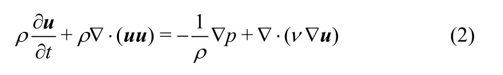
whereuis the velocity vector, (u,v) are the components of the velocity inx-,y-directions,respectively.ρis the density,tis the time,pis the pressure,νis the kinematic viscosity coefficient.

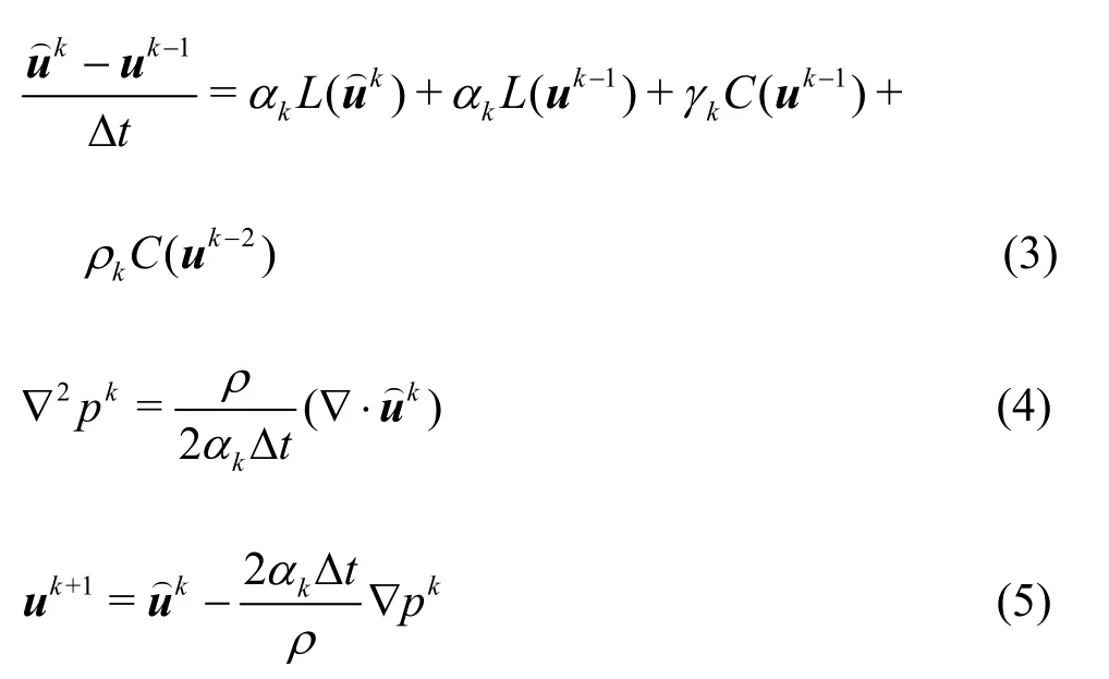
The N-S equations are discretized by a finite difference method on the staggered Cartesian grid.Also, the uncoupling of the pressure with the velocity is realized by a fractional step method[17].For the spatial discretization, the convective fluxes are handled by a Roeʼs flux difference splitting method with a high-order total variation diminishing monotonic upstream-centered scheme for conservation laws(TVD MUSCL) scheme[18].The central difference scheme is applied for the viscous fluxes.For the time advancement, a third-order Runge-Kutta method(RK3) is used for the integration of the momentum equations with the second-order Crank-Nicolson scheme.

1.2 Numerical implementation of the GCM

The GCM is used in the present study to consider the influence of the stationary and moving boundaries in the flow field.The boundary conditions on the interface are enforced by the use of the ghost cells.The ghost cells (GC) are defined as the cells in the solid adjacent to at least one cell in the fluid.The fluid cells (FC) are defined as the cells located in the fluid.The solid cells (SC) are the cells that are located in the solid with the ghost cells excluded.The ghost cell values are obtained by a bilinear interpolation method.The detailed treatment is explained as follows.In the GCM, the first key step is to describe and reconstruct the immersed boundaries, which is discussed in Section 1.3.The next step is to compute the ghost cell values by interpolation, to impose the boundary conditions.It consists of the following sub-steps:

(1) Mark the mirroring points: For each ghost cell, the mirroring points can be uniquely determined by mirroring the ghost cell values to the outside of the wall boundaries, as shown in Fig.1.The distance from mirroring points to projecting points of the wall boundary ΔLis artificially assigned as ΔL=[19], where dx, dyare the grid sizes alongx-,y-directions, respectively, to ensure that a mirroring point is close to a square region formed by four fluid cell centers which do not pass through the body surface.Therefore, the mirroring point values can be easily calculated by the bilinear interpolation scheme using the interpolation stencil of the four fluid cell centers.The coordinates of a mirroring point(xIP,yIP) are obtained as:

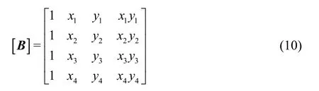
(2) Calculate mirroring point values by interpolation: Four fluid cells enclosing one mirroring point are the interpolation stencil points 1, 2, 3 and 4.The flow variableφof a mirroring point is expressed as

The unknown coefficient vector ［A]T=[a1a2a3a4]is determined by the variable values at the fluid nodes 1, 2, 3 and 4

where ［φ]= [φ1φ2φ3φ4]is the vector of the variable values at the fluid nodes 1, 2, 3 and 4.［]Bis the coefficients matrix of the bilinear interpolation scheme, which can be expressed as

After the coefficient vector ［A]is obtained by Eq.(9), the flow variableφof mirroring points can be calculated by Eq.(8).

Fig.1 Interpolation stencil in the GCM

(3) Calculate ghost cell values: the ghost cell valuesφGCcan be determined from the mirroring point valuesφIPin the fluid domain by interpolation

The velocity variables should satisfy the Dirichlet boundary condition, where,φBIis the velocity component of the projecting point,d1,d2are the distance from the ghost cell node to the projecting point and the distance from the projecting point to the mirroring point, respectively.The pressure variable should satisfy the Neumann boundary condition.The coefficients are obtained withξ1=1 andξ2=is the acceleration vector at the body surface.

In this way, the no-slip boundary conditions are satisfied when the N-S equations are solved by a standard five-point central-difference scheme in the entire computation domain.Consequently, the treatment for a complex moving body is simplified because the numerical discretization is not affected by the geometrical complexity of the immersed body.

1.3 Reconstructing interfaces by the PRBF

It is a big challenge accurately representing and tracking the immersed moving interfaces in the IBM,because the immersed boundaries are not inherently included in the computational grid.Here, the PRBF method is used to describe arbitrary complex boundaries.The key point is to fit an iso-surface function with some sampling points of the body surface.Then, the phase state of the background grid(fluid cells, solid cells and ghost cells) is identified by the sign of this iso-surface function.

For arbitrary immersed boundaries, the following field function is constructed by introducing the PRBF with a finite set of sampling data

whereNis the number of the offset points,is the variable value of one grid point,jβis the weight coefficient, the linear polynomial is expressed asthe kernel functionis expressed as

where the shape parameterCis a constant, which may be assigned asC=0.The weight coefficients of the PRBF should satisfy the following orthogonal condition

The weight coefficientjβcan be obtained by solving the following linear equations

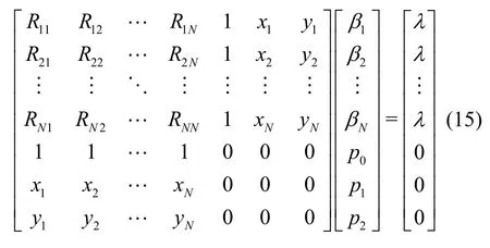
whereλis the iso-surface distance, which can be an arbitrary positive value, andλ=1 in the present study.Having known the weight coefficients, the field functiond(xi) can be obtained by Eq.(12).Thus,the iso-surface functionψ(x) can be formulated as

Thus, arbitrary geometries can be well described by the iso-surface functionψ(x).In the next step,three types of phase states on the background grid can be accurately identified by the use of the iso-surface functionψ(x), as shown in Fig.2.

Fig.2 Identifying the phase state of the background grid

Fig.3 Evolution history of the drag coefficients

Fig.4 Velocity profiles u ⋅Um ax-1 along the y-axis for three different phase angles

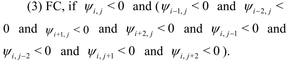
Then, by using the iso-surface functionψ(x),arbitrary geometries can be well described.To be consistent with the discretization stencils, we assign two layers of ghost cells to enforce the boundary conditions, as shown in Fig.2.The basic idea of the identification algorithm is to use the following properties of the PRBFψ.For a grid nodexi,j, ifψi,j＞0, then the nodexi,jis in the solid, ifψi,j＞0, then the nodexi,jis in the fluid, ifψi,j＞0,then the nodexi,jis on the body surface.Thus, the solid cells, the ghost cells and the fluid cells are identified in the following way:

2.Results and discussions

2.1 In-line oscillating of a circular cylinder

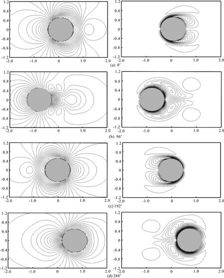
Fig.5 Pressure (left) and vorticity (right) contours at four different phase angles

A horizontally oscillating cylinder in a still fluid is simulated to examine the accuracy and the capability of the present method for moving boundary flows.The computational domain is set as [-10D,10D]×[- 8D, 8D]inx-,y-directions, respectively.The cylinder is in the origin of the Cartesian coordinates, where the diameter of the cylinder is set asD=1m.The Neumann velocity and the pressure boundary conditions are assumed on all boundaries.A constant time step is chosen as Δt = 0.005 s .To investigate the grid convergence, two kinds of grid systems (400×320 and 800×640) are used.The flow parameters are chosen based on the work of Guilmineau and Queutey[20].The Reynolds numberRe=UmaxD|νand the Keulegan-Carpenter numberKC=Umax/(fD) are two key flow parameters, which are set asRe= 100 andKC=5, respectively,whereUmaxis the maximum velocity of the cylinder withUmax=1m/s, andfis the oscillation frequency of the cylinder.A forced oscillation is described by a harmonic oscillation,x(t)=-Αs in(2 πft),U(t)=-Umaxcos(2 πft), whereΑis the amplitude of the oscillation.

The surface geometry of the cylinder could be fitted by the PRBF with a set of surface data.It could also be described by an analytic function as

whereRis the radius of the cylinder, (xo,yo) are the center coordinates of the cylinder.In the present study, both interface reconstruction methods mentioned above are used, and 100 sampling points of the body surface are used in the PRBF reconstruction method.

Figure 3 shows the evolution history of the drag coefficients by the proposed method with the PRBF and the analytic function reconstruction on two grid systems.The drag coefficients of the proposed method with both the PRBF reconstruction in Fig.3(a) and the analytic function reconstruction in Fig.3(b) agree well with those obtained by Guilmineau and Queuteyʼs body-fitted grid method on two grids.However, small high-frequency oscillations are observed on the coarse grid of 400×320 in both reconstruction strategies.The force oscillations are caused by the fact that the treatment of the moving boundary cannot fully maintain the local mass conservation in the Cartesian grid method.The oscillations can be reduced by refining the grid resolution.As seen in Fig.3, when the grid is refined to 800×640, much smooth drag coefficients are obtained with both reconstruction strategies.The oscillations can be also controlled by maintaining the local mass conservation on the moving boundary, which is not discussed here.Figure 4 shows the velocity profiles along they-axis at two locations (x=-0.6D,1.2D) for three phase angles(θ=180°, 210° and 330°) on the refined grid with the PRBF reconstruction.Again, good agreement is achieved when our results are compared with those from Guilmineau and Queutey.

The present method is further studied by analyzing the hydrodynamic characteristics of the flow field.In Fig.5, the snapshots of the instantaneous pressure and vorticity contours at four phaseangles are presented.Two stagnation points are symmetrically distributed at both ends of the cylinder,as shown in Fig.5(a).As the cylinder moves to the left, two counter-rotating vortices with the same length are generated, and the maximum pressure occurs, as shown in Fig.5(b).With the time advancement, the same process repeats on the second half of the period, as shown in Figs.5(c), 5(d).

2.2 Flow around a NACA0012 airfoil

Now, we focus on the numerical simulation of the flow around a NACA0012 airfoil.The computation is carried out at the domain [-3b,9b]×[-3b,3b]with a non-uniform grid of 600×400, wherebis the chord length,b=1m.The leading edge is located in the origin of the coordinates with an angle of attack of 0°.The geometry of the NACA0012 airfoil is described by the PRBF with 141 sampling points.The computational time step is chosen as Δt=0.001s .At the inflow boundary, a uniform flow is applied.The free flow and radiative boundary conditions are applied at the outflow boundary and freestream boundaries, respectively.The flow parameter is chosen according to Imamura et al.[21], the Reynolds numberRe=Umaxb|ν= 500.

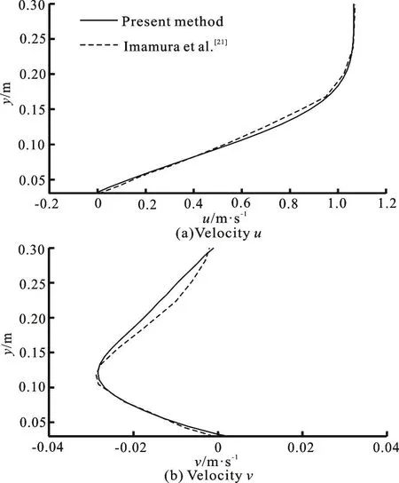
Fig.6 Boundary layer velocity profiles along the y-direction

The drag coefficient (CD=0.1653)obtained by the present method is slightly smaller than the value(CD=0.1725)from Imamura et al.on the finest grid,with errors within the tolerance.The good agreement shows that our CFD solver and PRBF method are accurate and reliable.Figure 6 shows the velocity profilesu,valongy-axis at the positionx=0.75m, respectively.The present results are in fair agreement with those of Imamura et al..The local differences may be due to the different interface treatments.In the present study, the no-slip boundary conditions are enforced by assigning the ghost cells in the solid domain.The pressure contours are shown at the Fig.7.The pressure is symmetrically distributed on the upper and lower surfaces, and a stagnation point is observed at the leading edge.

3.Conclusions

A ghost cell immersed boundary method is proposed to simulate the moving boundary flows.To track and reconstruct arbitrary complex geometries,the PRBF method is used for the interface description.To validate our CFD solver and interface representation method, two test cases are simulated.In the case of the in-line oscillation of a circular cylinder in the still fluid, the accuracy and the reliability of our ghost cell immersed boundary method is validated by comparing with the reference results.Also, the results of the present PRBF method well agree with those of the analytic function representation method.The second case is the uniform flow around an airfoil,which demonstrates the capacity of the PRBF method for the complex boundary.

We intent to extend the present method to the two-phase flow, to simulate complex moving boundaries interacting with free surface flow in a near future.