Xing-ya Xu (徐兴亚), Xuesong Zhang , Hong-wei Fang (方红卫), Rui-xun Lai (赖瑞勋),Yue-feng Zhang (张岳峰), Lei Huang (黄磊), Xiao-bo Liu (刘晓波)

1.Changjiang Institute of Survey, Planning, Design and Research, Wuhan 430010, China

2. State Key Laboratory of Hydroscience and Engineering, Department of Hydraulic Engineering, Tsinghua University, Beijing 100084, China

3.Joint Global Change Research Institute, Pacific Northwest National Laboratory, College Park, MD, USA

4.Great Lakes Bioenergy Research Center, Michigan State University, East Lansing, Michigan, USA

5.Yellow River Institute of Hydraulic Research, Zhengzhou 450003, China

6.Development Research Center of the Ministry of Water Resources of People’s Republic of China, Beijing 100038, China

7.Department of Water Environment, China Institute of Water Resources and Hydropower Research, Beijing 100038, China

Abstract: An accurate and reliable real-time flood forecast is crucial for mitigating flood disasters.The errors associated with the inflow boundary forcing data are considered as an important source of uncertainties in hydraulic model.In this paper, a real-time probabilistic channel flood forecasting model is developed with a novel function to incorporate the uncertainty of the forcing inflow.This new approach couples a hydraulic model with the particle filter (PF) data assimilation algorithm, a sequential Bayesian Monte Carlo method.The stage observations at hydrological stations are assimilated at each time step to update the model states in order to improve the next time stepʼs forecasting.This new approach is tested against a real flood event occurred in the upper Yangtze River.As compared with the open loop simulations, the evaluations of model performance with several deterministic and probabilistic metrics indicate that the accuracy of the ensemble mean prediction and the reliability of the uncertainty quantification are improved pronouncedly as a result of the PF assimilation.Further assessment of the prediction results at different lead times shows that the improvement of model performance deteriorates with the increase of the lead time due to the gradual diminishing of the updating effect for the initial conditions.Based on the analyses of the number of particles and the assimilation frequency, we find that the optimal number of particles can be determined by balancing the model performance and the computation cost, while a high assimilation frequency is preferred to incorporate the emerging observations to update the model states to match the real conditions.

Key words: Channel flood forecasting, probabilistic forecast, particle filter, hydraulic model, data assimilation, inflow uncertainty

Introduction

Flood is one of the most destructive natural disasters to human society, with serious losses of life and property every year[1].Flood forecasting is an important non-engineering measure for flood control by estimating a flood event in the future regarding the time of its occurrence, the quantitative measure and the reliability.The utility of a forecast increases by considering the predictive uncertainty to perform the probabilistic forecasting.Probabilistic flood forecasting assists flood managers so that they can make decisions by taking risks into account[2].

In hydraulic models, a robust characterization of the various uncertainties affecting the model output remains a major scientific and operational challenge[3].Generally, the hydraulic modeling is affected by four sources of uncertainty: (1) the forcing data uncertainty,e.g., the inflow discharge as a sequence of atmospheric and hydrologic model outputs, (2) the input uncertainty, e.g., due to the simplifications of the channel and floodplain topography or the model initial condition, (3) the structural uncertainty, arising from the lumped and simplified representation of the flood routing processes in hydraulic models, and (4) the parametric uncertainty, arising from the imperfect parameter calibration due to the finite length and the uncertainty of the historical observational data.Among these sources of uncertainty, the uncertainty of the forcing data (i.e., the inflow discharge from the upstream and the lateral flow) is significant and dominant[4].Research results show that, compared to the inflow discharge, other sources of uncertainty are negligible, so the errors in the inflow discharge are assumed as the only source of model errors in hydraulic models in some studies[5-6].

The data assimilation techniques can be used to update the estimates of the system states or parameters through quantifying errors in both the model and the observation, and therefore the accuracy of the model forecasts can be improved[7-8].Furthermore, theposteriordistribution of the model states and parameters can be estimated by the data assimilation techniques to reduce the uncertainty associated with the prior information.The particle filter (PF) is a sequential Monte Carlo data assimilation algorithm based on the Bayesian theory, which assigns a probability to each ensemble element by a weight calculation based on the difference between the ensemble element and the observation[9].The PF method were successfully applied to assimilate the observation data into the hydrological and hydraulic models to update the state variables, and has achieved significant reductions in the uncertainties of the flood forecasting[10-14].

In this study, we employ the PF method to assimilate the real-time stage data observed at the hydrological stations into the hydraulic model, as well as consider the uncertainty of the inflow discharge to improve the probabilistic flood forecasting performance.The rest of this paper is organized as follows.In the methodology section, the real-time probabilistic channel flood forecasting model by coupling a hydraulic model with the PF is described.The case study section includes the study river reach, the numerical experiment setup, the performance metrics,the results of the numerical experiment, and the discussions on the flood forecasting model performance.Finally, in the conclusion section, the conclusions of this study are summarized.

1.Methodology

1.1 Bayesian filtering theory

The evolution of a discrete-time dynamic statespace model can be formulated as follows:

wherexkandykare the vectors denoting the model and observation states at timek, respectively.The operatorfexpresses the model transition in response to the forcing datauk-1.The operatorhexpresses the observation function.θis the model parameter.ωk-1andvkrepresent the model and observation errors, respectively, andWk-1andVkrepresent the covariances of the errors.

From the perspective of the Bayesian filtering,the principal goal of the statexkestimation problem is to derive theposteriorprobabilistic distributionp(xk|y1:k) based on the available observational information.Theposteriordistribution can be estimated according to the Bayes law

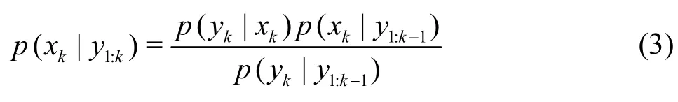
wherep(xk|y1:k-1) represents the prior distribution,p(yk|xk)represents the likelihood, andp(yk|y1:k-1) represents the normalizing constant.Assuming the model to be Markovian, the Bayes law can be applied recursively through the estimation of the prior distribution via the Chapman-Kolmogorov equations,as follows

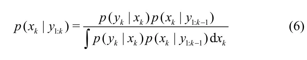
The prior distribution is derived through the integration of the transition probabilityp(xk|xk-1)and theposteriordistribution at the previous time stepp(xk-1|y1:k-1).The likelihood is typically calculated by a normal likelihood function.The normalizing constant can be expanded to the integral of the total probability, using the states as the intermediate variables

Substituting Eqs.(4), (5) into Eq.(3), theposteriordistribution can be computed sequentially in time as

As most dynamic state-space models are nonlinear, the analytical solutions are intractable.The numerical methods, such as the PF method, are used for solving the Bayesian filtering problem.

1.2 Particle filter

The PF is an approximation method to solve the Bayesian filtering problem by the Monte Carlo sampling.The key idea of the PF is to represent the probabilistic distribution by a set of random samples, called the particles, with associated weights.When the number of particles is large enough, the probabilistic distribution can be approximated by the ensemble of the particles.Theposteriorprobabilistic distribution function can be described as

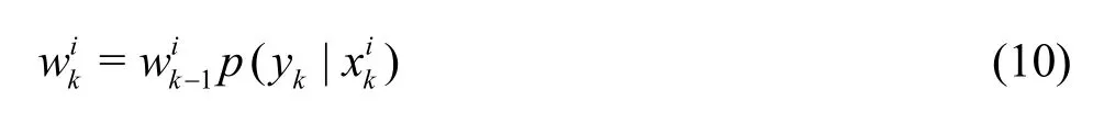
The selection of the importance density is an important issue as it significantly influences the filter performance.Generally, the transition prior distribution is used as the proposed distribution, where

Substituting Eq.(9) into Eq.(8), the weight updating is simplified to

However, there is a common problem with respect to the PF called the “particle degeneracy”, i.e.,most particles have negligible weights after a few iterations[11].A great computational effort is devoted to updating the particles with contributions of nearly zero to approximate theposteriordistribution.Here,resampling is applied to solve this problem, and the basic idea is to eliminate the particles with small weights while multiply the particles with large weights.There are various resampling methods, and the most commonly used methods are the multinomial resampling, the stratified resampling, the systematic resampling and the residual resampling.Specially, the residual resampling method is used in this study because it can effectively reduce the variances of the particle weights and is computationally more efficient than other resampling methods.After resampling, all particles are assigned with the same weight, that isFinally, theposteriordistribution can be approximated as follows

The sequential importance resampling (SIR) is a PF method that resamples the particles at each analysis step.The SIR was applied widely in many studies[8-16], and will be implemented in this study.

1.3 Hydraulic model with the particle filter

The hydraulic model employed here is a 1-D unsteady open-channel flow model represented by the Saint-Venant formulation as:

whereQis the discharge,Zis the stage,Ais the cross-section area,Ris the hydraulic radius andqlis the lateral discharge, andnis the Manning roughness coefficient.

There are two flow state variables (i.e., the dischargeQand the stageZ) and one parameter(i.e., the Manning roughness coefficientn) in the Saint-Venant formulation.Equations (12), (13) are hyperbolic partial differential equations and can be numerically solved with the four-point implicit finitedifference approximation with appropriate initial and boundary conditions[17].The initial conditions are the discharge and the stage on every cross-section at the initial time.The inflow discharges from the upstream and the lateral flow, and the stages in the downstream are served as the boundary conditions.

As mentioned in introduction, the uncertainty of the inflow discharge is the main source of the uncertainty of the hydraulic modelʼs output.With the incorporation of the uncertainty of the inflow discharges into the hydraulic models, the probabilistic forecasting can be performed.To better estimate the uncertainty of the inflow discharge and improve the quality of the probabilistic forecasting, the real-time hydrological observations obtained from the hydrological stations along the channel are employed to be assimilated into the hydraulic model using the PF.

According to the PF theory, a basic particle representing a realization of the stochastic flow in the flood forecasting model is defined as:

where m is the total number of the channel cross sections.

The ensemble of all particles can approximate the probabilistic distribution of the flood flow and provide a means for the uncertainty estimation.For the observed stage data are much more accurate than the observed discharge data, only the real-time stage observations are used in the assimilation analysis step.The likelihood is calculated against the stage observations of each hydrological station in the normal likelihood function as

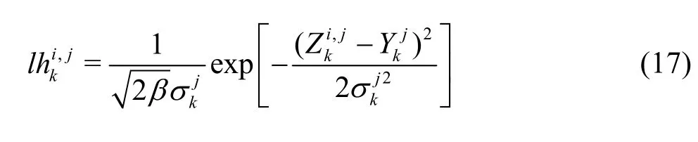
The overall likelihood of a particle is calculated by applying the joint probability theory for independent variables

where Nois the number of the hydrological stations.

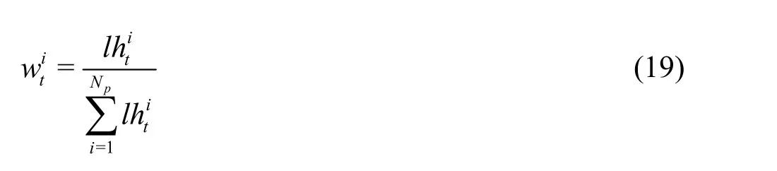
Then the weight of each particle can be derived by normalization

The technical process of the flood forecasting model with the PF assimilation is schematically displayed in Fig.1.Additionally, the procedures are summarized as follows:

(1) At the initial time k=0, Npparticles with equal weights are sampled from the prior distribution of the state variables :1/Np.

(2) The particles are propagated through the hydraulic model to forecast the flood under the uncertain forcing inflow discharges, and the forecasted particles are obtained as:

(3) If the new stage observations are available,the likelihood of each particle can be calculated.The normalized particle weights can be subsequently derived as:if they fall into tolerated limits, go to (4).otherwise, go to (5).

(4) Resample the particles with the residual resampling technique.The particles are updated to new ones with equal weights:

(5) If all time steps finish, the whole process stops.Otherwise, k=k+1, and go back to (2).

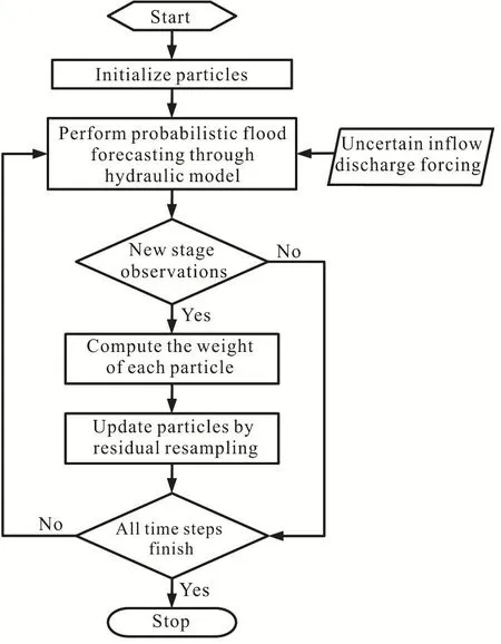
Fig.1 Flow chart of the probabilistic flood forecasting model with the PF assimilation

2.Case study

2.1 Study area

The study area locates in the river reach from Cuntan to Zhongxian in the Three Gorges of the Yangtze River, China (Fig.2).The mainstream channel length from Cuntan to Zhongxian is about 228 km with a gradient of 0.003%-0.270%.During summer and fall, the torrential rain falling on the steep mountains of the Three Gorges region can lead to damaging fast-flowing floods.There are two intermediate hydrological stations in the study channel, i.e.,the Changshou and Qingxichang stations, where the real-time hydrological observations are transmitted to the flood control center instantly.The calibrated Manning roughness coefficients along the study channel are 0.036 from Cuntan to Changshou, 0.040 from Changshou to Qingxichang, and 0.035 from Qingxichang to Zhongxian[18].

Fig.2 River reach of the Yangtze River from Cuntan to Zhongxian

2.2 Experiment setup

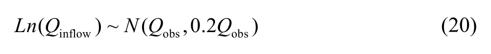
To test the usefulness and the effectiveness of the developed flood forecasting model, numerical experiments are carried out to simulate the historical flood events.A typical real flood event with a return period of about 20 years is selected as the scenario for the simulation.The flood event is from June 27, 2009 to July 09, 2009, during which time, the stages at Changshou and Qingxichang stations were recorded every hour.The inflow discharge forcing data for the hydraulic model is supposed to be the basin outflow above Cuntan, which can be provided by an atmospheric precipitation and hydrological rainfall-runoff model.However, the output uncertainty of the specific atmospheric and hydrological models is beyond the study scope of this paper.Instead, the uncertainty of the inflow discharge for the hydraulic model is represented by perturbing the historical observed inflow discharge data at Cuntan station as stochastic variables.According to previous studies[3,19], the multiplicative log-normal noises are applied as the nominal observed values

With both the computational efficiency and the assimilation effectiveness in mind, the number of particlesNpis selected as 100 in the experiment,which will be discussed in the following part of this paper.Each particle is driven by a random inflow discharge to perform the flood forecasting at multiple lead times.For every hour, when the new stage observations at Changshou and Qingxichang stations are available, the PF assimilation analysis is made.

2.3 Performance metrics

To provide a robust analysis, the metrics are selected to quantitatively evaluate the model performance with respect to both the accuracy and the reliability[20-21].

The model performance in the accuracy is evaluated by three deterministic quantitative measures:the Nash-Sutcliffe efficiency (NSE), the root mean square error (RMSE), and the mean bias (MB), which are defined as follow:

whereykis the stage observation at timek,is the mean of all available observations,is the ensemble mean of the particle predictions at timek,andTis the total number of available observations.

The model performance in the reliability is evaluated by three probabilistic quantitative measures:the normalized root-mean-square error ratio (NRR),the rank histogram, and the Quantile-Quantile plot(QQ plot).

The NRR is a normalized measure of the ensemble dispersion indicating how confidently the ensemble mean can be extracted from the ensemble spread[22].

whereR1is the time-averaged RMSE of the ensemble mean,R2is the mean RMSE of the ensemble members,E(Ra) is the expected ratio ofR1toR2when the observation is statistically indistinguishable from a member of the ensemble, which is

It is expected that the model performance has a perfect reliability when NRR=1.However, NRR＞1 indi- cates that the ensemble has too little spread,while NRR＜1 is an indication of an ensemble with too much spread.

The rank histograms describe the probability that an observation falls into the intervals defined by the sorted prediction ensembles.The rank of the observation at timekcan be calculated according to the following equation.

Similar to the rank histogram, a QQ plot is used to diagnose errors in the prediction distribution.A QQ plot is created by first calculating the normalized rank of each observation.

Then the plot compares the normalized rank ony-axis and the uniform distribution onx-axis to examine the reliability of the prediction distribution.If the plot follows the 1:1 line, this prediction is perfectly reliable.If the predictive QQ line falls above the 1:1 line, the prediction has a low bias (observations have a tendency to take higher values in the prediction distribution) and a predictive QQ line falling below the 1:1 line indicates a high bias.In addition to the bias, the overconfidence or underconfidence of a prediction distribution can be diagnosed with the QQ plot.If the predictive QQ line falls above the left side of the 1:1 line and crosses the 1:1 line in the middle,the prediction is over confident (a disproportionately large number of observations being captured by outer quantiles of the prediction distribution) and the reverse case indicates the prediction is under confident.The supportive quantitative scores are also included in the QQ plot:

whereUis the normalized uniform cumulative density,E[]is an expected value operator andSD[]is a standard deviation operator.

With respect to the reliability of the prediction,αis a measure of the uniformity of the QQ plot (i.e.,α= 0 represents the worst situation while 1 is the perfect score) andβis a measure of the resolution of the prediction.If two predictions have a similar reliability, the prediction with a greater resolution is preferred because it enjoys a lower level of uncertainty.

2.4 Results

2.4.1 Assimilation performance

Figure 3 shows the comparison of the probabilistic stage hydrographs in the flood event between the open loop (without assimilation) and the PF assimilation simulations at Changshou and Qingxichang.It is apparent that after the assimilation using the PF, the ensemble mean stages become closer to the observations, and the prior 95% confidence interval becomes much narrower, with an increased reliability of the confidence interval.

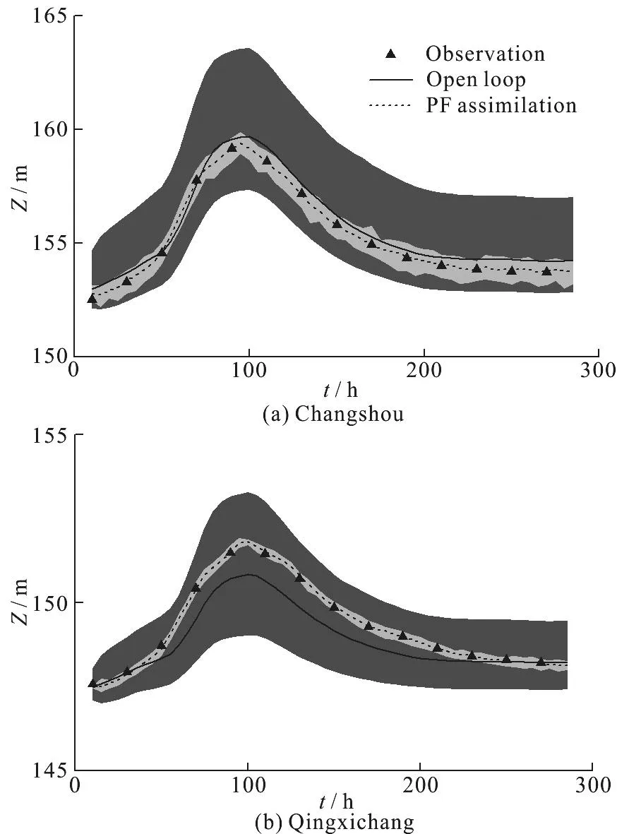
Fig.3 Probabilistic stage hydrographs in the open loop and the PF assimilation simulations.(The lines represent the ensemble mean in the open loop (solid) and the PF assimilation (dashed) simulations.The shaded areas correspond to 95% confidence intervals in the open loop (dark shading) and the PF assimilation (light shading) simulations)

To illustrate the updating process of the particles,Fig.4 shows the frequency histograms of the prior predicted stages and theposteriorupdated stages, i.e.,the stages before and after the assimilation at 12:00 June 29 (t= 60h) in the rising limb of the hydrograph, at Changshou and Qingxichang, respectively.As it is assumed that the weights of individual particles depend on the distance from the observation,the particles closer to the observation are specified with higher weights and more likely to be duplicated in the resampling process.After the assimilation, the histogram centroid at Changshou moves from 154.29 m to 154.62 m with an observed stage value of 154.70 m and the histogram centroid at Qingxichang moves from 148.43 m to 148.58 m with an observed stage value of 154.53 m.This result clearly indicates that the ensemble mean value becomes closer to the observation after the process of the PF assimilation.In addition, the range of the histogram at Changshou is narrowed from 153.0-156.0 m to 154.0-155.5 m, and the range of the histogram at Qingxichang is also narrowed from 148.1-148.9 m to 148.4-148.8 m,showing that the spreads of the uncertainty are pronouncedly reduced.

Fig.4 Histograms of prior (gray) and posterior (dashed) distributions of stages at t=60h (The observed stages are indicated as stars.The vertical dash line indicates the histogram centroid of prior distribution and the vertical solid line indicates the histogram centroid of posterior distribution)

Fig.5 Probabilistic inflow hydrographs at Cuntan.(The shaded areas correspond to 95% confidence intervals by the open loop (dark shading) and the PF assimilation (light shading) simulations.The dots represent observed discharges)

Since the two state variables, the discharge and the stage, are coupled closely in the hydraulic model,the discharge is also updated indirectly with the stage after the stage observations are assimilated.Figure 5 shows the uncertainty of the inflow discharge in the open loop and the PF assimilation simulations.Based on the limited prior information, the uncertainty of the inflow discharge is quite large in the open loop simulation.After the stage observations are assimilated, the uncertainty of the inflow discharge is reduced effectively to a reasonable interval.

Fig.6 Performance metrics in the open loop and the PF assimilation simulations

Fig.7 Rank histograms in the open loop and the PF assimilation simulations

Fig.8 QQ plots in the open loop and the PF assimilation simulations

The deterministicandprobabilisticmetricsare calculated to evaluate the accuracy and the reliability of the model performance in the open loop and the PF assimilation simulations, as shown in Fig.6.

Fig.9 Probabilistic stage hydrographs at forecast lead times of 3 h, 6 h, 9 h and 12 h

With respect to the deterministic metrics, the model performance in the PF assimilation simulation features a higher NSE value and lower RMSE and MB values than those in the open loop simulation.Specifically, the NSE value increases from 0.82 to 0.97 at Changshou and from 0.91 to 0.99 at Qingxichang, the RMSE value decreases from 0.42 to 0.05 m at Changshou and from 0.31 to 0.03 m at Qingxichang,and the MB value decreases from 0.16 to 0.03 m at Changshou and from 0.11 to 0.02 m at Qingxichang.The results of the deterministic metrics indicate that the accuracy of the model performance is improved effectively after the PF assimilation.

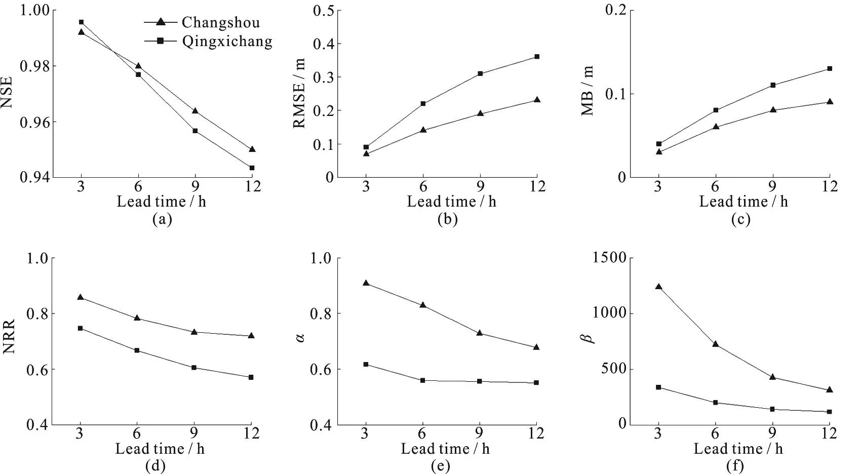
Fig.10 Forecasting performance metrics at forecast lead times of 3 h, 6 h, 9 h and 12 h

In terms of the probabilistic metrics, the NRR values in the open loop simulation (0.41 at Changshou and 0.56 at Qingxichang) are much lower than 1,indicating that the ensemble spread is too wide.After the PF assimilation, the NRR values turn towards 1,with 0.88 at Changshou and 0.95 at Qingxichang,indicating that the reliability of the ensemble is increased significantly.The rank histograms and the QQ plots illustrate the probabilistic distributions of the uncertainty, as shown in Figs.7, 8.In the open loop simulation, it is observed that a large portion of observations fall into the middle bins of the rank histogram at Changshou, indicating an underconfidence case.However, most observations fall into the right bins of the rank histogram at Qingxichang,indicating a bias of underestimation.Compared to the open loop simulation, the PF assimilation simulation results in more uniform rank histograms, implying more reliable representations of the uncertainty.A similar result is produced by the QQ plots.After the PF assimilation, the QQ lines move closer to the 1:1 line, withαvalues increasing from 0.57 to 0.79 at Changshou and from 0.55 to 0.96 at Qingxichang.Meanwhile,βvalues also increase from 96.60 to 209.26 at Changshou and from 638.68 to 2295.27 at Qingxichang, indicating more reliable and precise distributions of the uncertainty.

Overall, the metrics examined here show the usefulness and the effectiveness of the PF assimilation in improving the accuracy and the reliability of the model performance.

2.4.2 Forecasting performance

After the PF assimilation, the real-time probabilistic flood forecasting at different forecast lead times are performed by the hydraulic model with the prior known inflow discharge as the boundary forcing data.

Figure 9 shows the predicted probabilistic stage hydrographs against the observations at Changshou and Qingxichang at different forecast lead times, i.e.,3 h, 6 h, 9 h and 12 h.Compared to the model performance in the open loop simulation shown in Fig.3,the forecasting performance is improved significantly with a higher accuracy and reliability in the PF assimilation simulation.Notably, as the forecast lead time increases, the level of the model improvement decreases with a wider associated 95% uncertainty interval.

The deterministic and probabilistic metrics listed above are also used to evaluate the accuracy and the reliability of the forecasting performance quantitatively, as shown in Figs.10, 11.

With respect to the deterministic metrics, it is observed that when the forecast lead time increases from 3 h to 12 h, the NSE value decreases from 0.99 to 0.94 at Changshou and from 0.99 to 0.95 at Qingxichang, the RMSE value increases from 0.09 to 0.36 m at Changshou and from 0.07 to 0.23 m at Qingxichang, and the MB value increases from 0.04 to 0.13 m at Changshou and from 0.03 to 0.09 m at Qingxichang.

Regarding the probabilistic metrics, it is observed that when the forecast lead time increases from 3 h to 12 h, the NRR value decreases from 0.75 to 0.57 at Changshou and from 0.86 to 0.72 at Qingxichang,αvaluedecreases from 0.62 to 0.55 at Changshou and from 0.91 to 0.68 at Qingxichang, andβvalue decreases from 337.59 to 116.52 at Changshou and from 1 236 to 311 at Qingxichang.In addition, as the forecast lead time increases, the QQ plot lines deviate further away from the 1:1 line gradually.

These indicate that when the forecast lead time increases, the effects of updating the model initial conditions by the PF assimilation on the predicted results gradually diminish, resulting in the deterioration of the accuracy and the reliability of the model forecasting performance.If the forecast lead time is long enough, the improvement by the PF assimilation will disappear eventually.Similar results are also reported in previous studies[6,15].

Fig.11 (Color online) QQ plots at forecast lead times of 3 h, 6 h,9 h and 12 h

2.4.3Analysis of number of particles and assimilation frequency

In this section, the effects of two important factors, the number of particles and the assimilation frequency, on the model performance are investigated by numerical experiments.

In order to evaluate the performance with respect to different numbers of particles, six particle sets (40,60, 80, 100, 200 and 500) are considered in the numerical experiment.Figure 12 shows the RMSE and NRR values of the assimilation performance with different numbers of particles.The trend is obvious that with the increase of the numbers of particles, both the accuracy and the reliability of the model performance are improved.More particles can lead to more accurate estimation and more reliable uncertainty quantification, however, at the expense of more computation resource.Thus, it is necessary to analyze the tradeoff between the performance quality and the computation resource cost.In this case, when the number of particles goes beyond 100, the model performance begins to level off.Employing more particles could not significantly improve the model performance, with unnecessary computational cost.

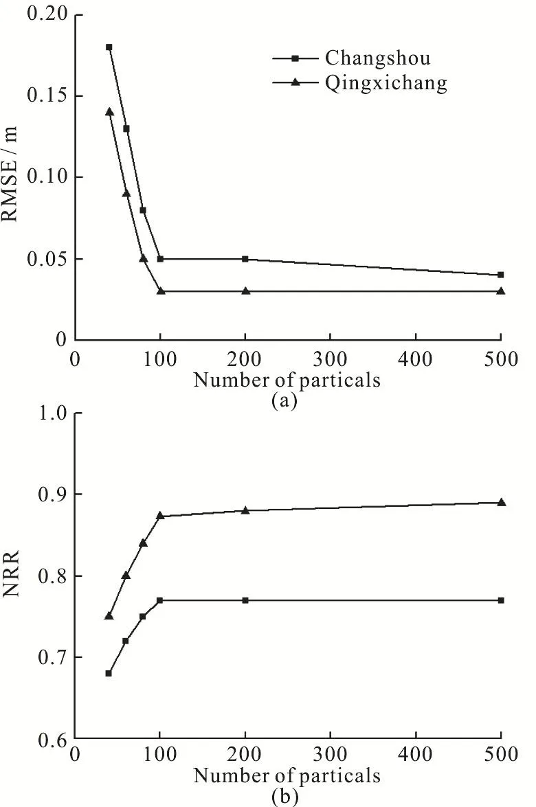
Fig.12 Assimilation performance with different numbers of particles

The assimilation frequency means how often the observation data become available to be assimilated into the model.In order to evaluate the performance with respect to different assimilation frequencies,three time intervals (3 h, 6 h and 12 h) are set as the assimilation interval in the experiment.Similar to the analysis of the number of particles, the RMSE and NRR values of the assimilation performance with different assimilation frequencies are shown in Fig.13.According to the results, the increase of the assimilation frequency improves the model performance in both accuracy and reliability.With a higher assimilation frequency, the observation information can be incorporated into the model to update the state variables more timely.Therefore the instantaneous changes of the unsteady flood flow can be better characterized by the model.Thus, if it is feasible with the automatic hydrological monitoring and information transmission technologies, a high assimilation frequency is preferred to improve the real-time flood forecasting performance.

Fig.13 Assimilation performance with different assimilation frequencies

3.Conclusion

In this study, we develop and evaluate a real-time probabilistic channel flood forecasting model approach by incorporating the uncertainty of the forcing inflow discharge.In the developed model approach,the stage observations are assimilated into the hydraulic model with the PF to update the state variables.A case study of a real flood event occurred in the upper Yangtze River reach is used to test the model, and several quantitative deterministic and probabilistic metrics are introduced to evaluate the accuracy and the reliability of the model performance.The evaluation results of the assimilation performance show that the PF assimilation can update the state variables from the prior distributions to theposteriordistributions effectively.The accuracy of the ensemble mean prediction and the reliability of the uncertainty intervals are significantly improved after the PF assimilation over those in the open loop simulation.The evaluation results of the forecasting performance with lead times of 3 h, 6 h, 9 h and 12 h show that the model forecasting for a shorter lead time has more accurate and reliable performance, i.e.the model performance will decrease with the increase of the lead time due to the gradual diminishing of the updating effect on the initial conditions.The examination of different numbers of particles shows that the optimal number of particles can be chosen as a tradeoff between the model performance and the computation cost.The analysis of the assimilation frequency indicates that a higher assimilation frequency can help to improve the model performance by updating the model states more timely to better represent the instantaneous condition of the unsteady flood.

Acknowledgements

This research was supported by the NASA New Investigator Award (NIP, NNH13ZDA001N) and Terrestrial Ecology Program (NNH12AU03I) as part of the North American Carbon Program, and the DOE Great Lakes Bioenergy Research Center (DOE BER Office of Science DE-FC02-07ER64494, DOE BER Office of Science KP1601050, DOE EERE OBP 20469-19145).