WANG Li-wei,SHU Li-sheng

(1.School of Mathematics and Physics,Anhui Polytechnic University,Wuhu 241000,China)

(2.School of Mathematics and Computer Science,Anhui Normal University,Wuhu 241003,China)

Abstract:In this paper,we study the boundedness of multilinear commutators of the Littlewood-Paley operators in variable exponent Lebesgue spaces.Based on the atomic decomposition and generalization of the BMO norms,we also prove some boundedness results for such multilinear commutators in variable exponent Herz-type Hardy spaces,which essentially extend some known results.

Keywords:Littlewood-Paley operators;variable exponent;Herz-type Hardy spaces;commutators

1 Introduction

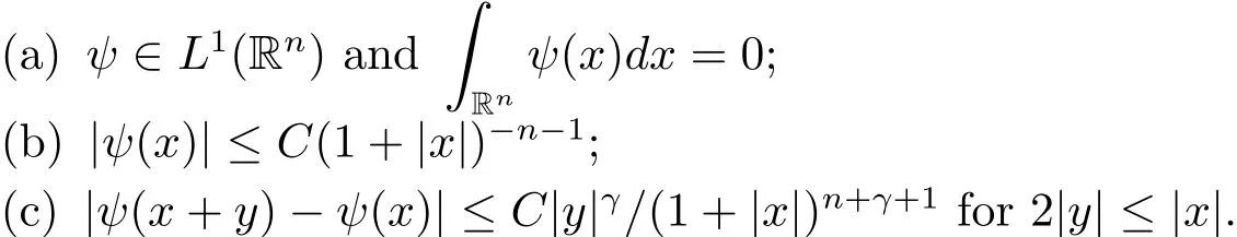
Let ψ be a function on Rnsuch that there exist positive constants C and γ satisfying

For this ψ andµ ＞1,the Littlewood-Paley’sfunction is defined by

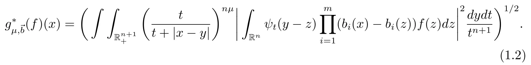
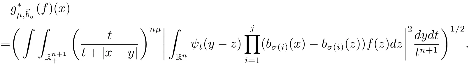
Given a positive integer m and a vector →b=(b1,b2,···,bm)of locally integrable functions,motivated by the work of Pérez and Trujillo-González[1]on multilinear operators,we define multilinear commutators of the Littlewood-Paley’sfunction as follows:

In the case of m=1,we usually denoteby

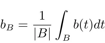
A locally integrable function b is said to be a BMO function,if it satisfies

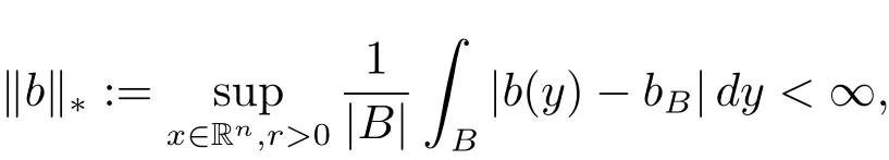
where and in the sequel B is ball centered at x and radius of r,

and ‖b‖∗is the norm in BMO(Rn).For bi∈ BMO(Rn),i=1,2,···,m,Xue and Ding[2]established the weighted Lpand weighted weak L(logL)-type estimates for the multilinear

In recent years,following the fundamental work of Kováčik and Rákosník[7],function spaces with variable exponent,such as variable exponent Lebesgue and Herz-type Hardy spaces etc.,have attracted a great attention in connection with problems of the boundedness of classical operators on those spaces,which in turn were motivated by the treatment of recent problems in fluid dynamics,image restoration and differential equations with p(x)-growth,see[8–16]and the references therein.

Karlovich and Lerner in[17]showed that[b,T],the commutator of a standard Calderón-Zygmund singular integral operator T and a BMO function b,is bounded on Lp(·)(Rn),which improved a celebrated result by Coifman et al.in[18].Recently,Xu[19]made a futher step and proved that the multilinear commutators T→b,a generalization of the commutator[b,T],enjoy the same Lp(·)(Rn)estimates when bi∈ BMO(Rn),i=1,2,···,m.These results inspire us to ask whether the multilinear commutators g∗µ,→bhave the similar mapping properties in variable exponent spaces Lp(·)(Rn)?Our first result(see Theorem 3.1 below)will give an affirmative answer to this question.

The variable exponent Herz spacesandwerefirst studied by Izuki[20,21].Simultaneously,he gave some basic lemmas on generalization of the BMO norms to get the boundedness of classical operators on such spaces.On the other hand,the variable exponent Herz-type Hardy spaces,as well as their atomic decomposition characterizations,were intensively studied by a significant number of authors[22,23].Using these decompositions,they also established the boundedness results for some singular integral operators.Motivated by the results mentioned above,another purpose of this article is to study the boundedness ofin variable exponent Herz-type Hardy spaces,which improves the corresponding main result in classical case(see[3,Theorem 2]).

In general,we denote cubes in Rnby Q.If E is a subset of Rn,|E|denotes its Lebesgue measure and χEdenotes its characteristic function.For l∈ Z,we define Bl={x ∈ Rn:|x|≤ 2l}.p′(·)denotes the conjugate exponent defined by 1/p(·)+1/p′(·)=1.By S′(Rn),we denote the space of tempered distributions.We use x≈y if there exist constants c1,c2such that c1x≤y≤c2x,C stands for a positive constant,which may vary from line to line.

2 Preliminaries and Lemmas

We begin with a brief and necessarily incomplete review of the variable exponent Lebesgue spaces Lp(·)(Rn),see[24,25]for more information.

Let p(·):Rn→ [1,∞)be a measurable function.We assume that

where and in the sequel

By Lp(·)(Rn)we denote the set of all measurable functions f on Rnsuch that

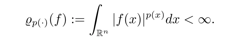
This is a Banach space with the norm(the Luxemburg-Nakano norm)

Given an open set Ω ⊂ Rn,the spaceis defined by

For the sake of simplicity,we use the notation

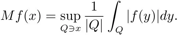
where M is the Hardy-Littlewood maximal operator defined by

When p(·) ∈ P(Rn),the generalized Höolder inequality holds in the form

with rp=1+1/p−−1/p+,see[7,Theorem 2.1].

We say a measurable function φ :Rn→ [1,∞)is globally log-Höolder continuous if it satisfies

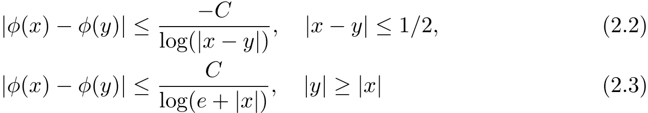
for any x,y ∈ Rn.The set of p(·)satisfying(2.2)and(2.3)is denoted by LH(Rn).It is well-known that if p(·) ∈ P(Rn)TLH(Rn),then the Hardy-Littlewood maximal operator M is bounded on Lp(·)(Rn),thus we have p(·) ∈ B(Rn),see[24].

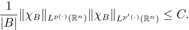
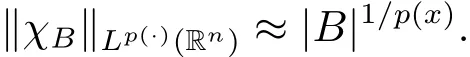
Lemma 2.1(see[21])Suppose p(·) ∈ B(Rn),then we have

Lemma 2.2(see[21])Suppose p(·) ∈ B(Rn),then we have for all measurable subsets E⊂B,

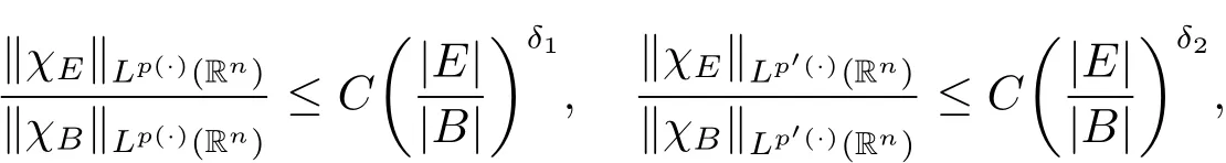
where δ1,δ2are constants with 0 ＜ δ1,δ2＜ 1.

Remark 2.1 We would like to stress that everywhere below the constants δ1and δ2are always the same as in Lemma 2.2.

Lemma 2.3(see[24])Suppose pi(·),p(·) ∈ P(Rn),i=1,2,···,m,so that

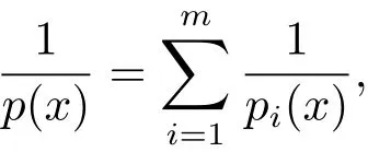
where m ∈ N.Then for all fi∈ Lpi(·)(Rn),we have

Lemma 2.4(see[25])Suppose p(·)∈ LH(Rn)and 0＜ p−≤ p(x)≤ p+＜ ∞.

(i)For all balls(or cubes)|B|≤2nand any x∈B,we have

(ii)For all balls(or cubes)|B|≥1,we have

Combining Lemma 2.3,Lemma 2.4 and Lemma 3 in[21,page 464],a simple computation shows that

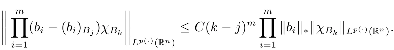
Lemma 2.5 Suppose p(·) ∈ P(Rn)TLH(Rn),bi∈ BMO(Rn),i=1,2,···,m,k ＞j(k,j∈N),then we have

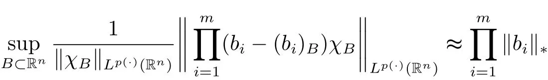
and

Remark 2.2 We note that Lemma 2.5 generalizes the well known properties for BMO(Rn)spaces(see[26]),and is also a generalization of Lemma 3 in[21].

3 Boundedness on Variable Exponent Lebesgue Spaces

We first recall some pointwise estimates for sharp maximal functions,the duality and density in variable exponent Lebesgue spaces Lp(·)(Rn).

For p(·) ∈ P(Rn),the spaces Lp(·)(Rn)can be endowed with the Orlicz type norm

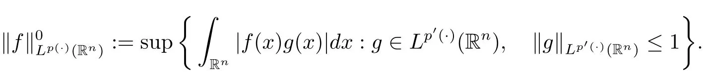
This norm,as pointed out in[7],is equivalent to the Luxemburg-Nakano norm,that is

where rp=1+1/p−−1/p+.

Proposition 3.1 Suppose p(·)∈ P(Rn),thenis dense in Lp(·)(Rn)and in Lp′(·)(Rn).For δ＞ 0 and f ∈(Rn),we define

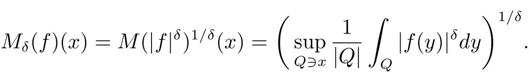
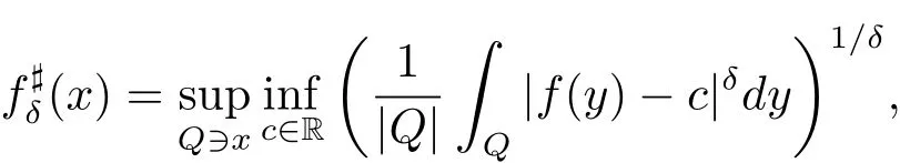
where the supremums are taken over all cubes Q⊂Rncontaining x.

The non-increasing rearrangement of a measurable function f on Rnis defined as

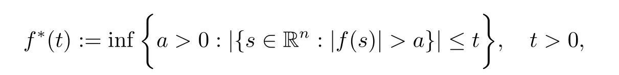
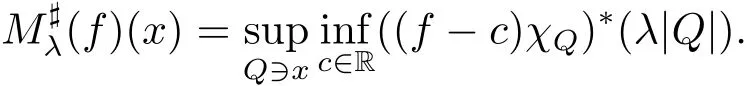
and for a fixed λ∈(0,1),the local sharp maximal functionis given by

The next lemma is due to Karlovich and Lerner[17,Proposition 2.3].

Lemma 3.1 Suppose λ ∈ (0,1),δ＞ 0 and f ∈(Rn),then we have

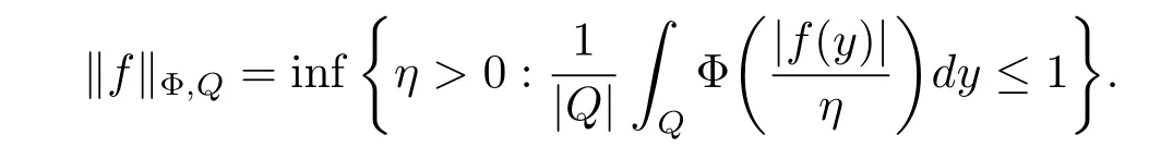
A function Φ defined on[0,∞)is said to be a Young function,if Φ is a continuous,nonnegative,strictly increasing and convex function withWe define the Φ-average of a function f over a cube Q by

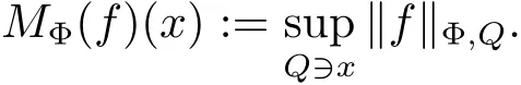
Associated to this Φ-average,we define the maximal operator MΦby

When Φ(t)=tlogr(e+t)(r ≥ 1),we denote MΦby ML(logL)r.It is well-known that if m∈N,then ML(logL)m≈Mm+1,the m+1 iterations of the Hardy-Littlewood maximal operator M,see[1].

Lemma 3.2(see[2])Let 0＜δ＜1.Then there exsits a positive constant C,independet of f and x,such thatx∈Rnholds for all bounded function f with compact support.

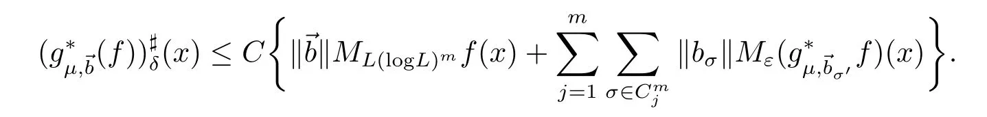
In fact,there holds a similar piontwise estimate for the multilinear commutatorsTo state it,we first introduce some notations.

As in[1],given any positive integer m,for all 1≤j≤m,we denote bythe family of all finite subset σ ={σ(1),σ(2),···,σ(j)}of{1,2,···,m}of j different elements.For any σ ∈,we associate the complementary sequence σ′given by σ′={1,2,···,m}σ.

For any σ ={σ(1),σ(2),···,σ(j)} ∈,we define

In the case σ ={1,2,···,m},we understandand

We now mention an immediate consequence of Proposition 2.4 in[2].

Lemma 3.3 Supposeµ＞2 and 0＜δ＜ε＜1.Then for any f∈,there exists a constant C ＞ 0,depending only on δ and ε,such that

We also need the following result from Lerner[27,Theorem 1].

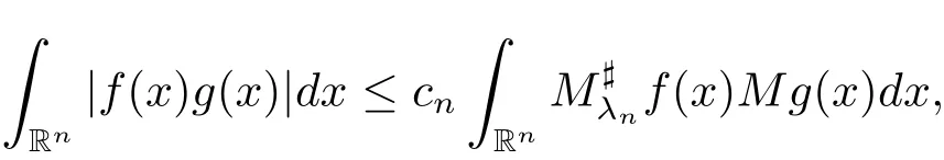
where constants 0＜λn＜1 and cndepend only on dimension n.

To prove Theorem 3.1,we first prove the following result which has its independent role.

Lemma 3.5 Supposeµ ＞ 2 and 0＜ γ ＜ min{(µ −2)n/2,1}.If p(·)∈ B(Rn),thenis bounded from Lp(·)(Rn)to itself.

Here for the last inequality we have used the fact that if p(·) ∈ B(Rn),then p′(·) ∈ B(Rn),see[21,Proposition 2].Thus we have

By Proposition 3.1,this concludes the proof of Lemma 3.5.

We now state the main result of this section.

Theorem 3.1 Supposeµ＞2,0＜γ＜min{(µ−2)n/2,1}and bi∈BMO(Rn),i=1,2,···,m.If p(·)∈ B(Rn),thenare bounded from Lp(·)(Rn)to itself.

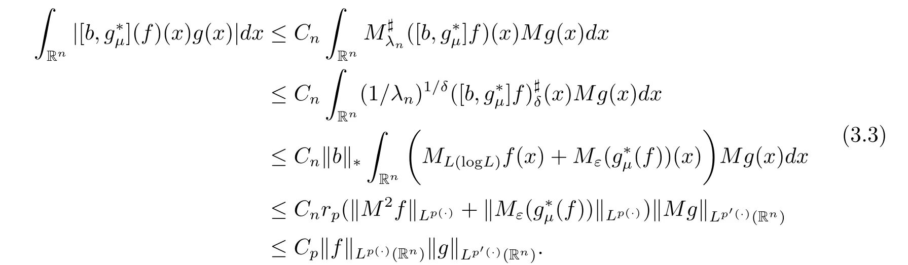
This together with(3.1)yields

Suppose now that the Theorem 3.1 is true for m−1.We will show that it is true for m.Once again by Theorem 1.2 in[2],according to Lemmas 3.4,3.1,3.2 and the generalized Höolder inequality(2.1),we have

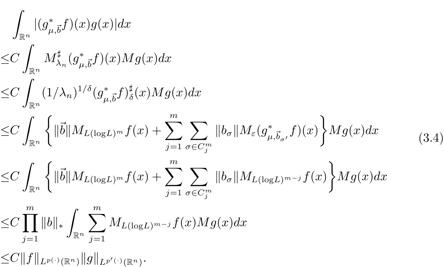
Now we obtain from(3.4)and(3.1)that

By Proposition 3.1,this concludes the proof of Theorem 3.1.

4 Boundedness on Variable Exponent Herz-Type Hardy Spaces

The main purpose of this section is to further study the mapping properties of the multilinear commutatorsin variable exponent Herz-type Hardy spaces.Before stating the main result,we give some definitions.

Let

and χk= χRkbe the characteristic function of the set Rkfor k ∈ Z.

Definition 4.1 Let p(·)∈ P(Rn),0 ＜ q ≤ ∞ and α ∈ R.The homogeneous variable exponent Herz spaceconsists of allsatisfying

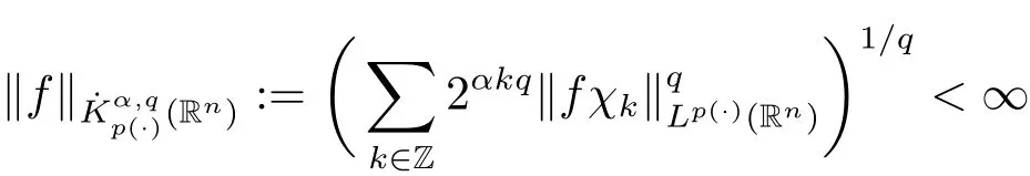
with the usual modification when q=∞.

For x∈R,we denote by[x]the largest integer less than or equal to x.

Definition 4.2 Suppose α ≥ nδ2,p(·) ∈ P(Rn)and non-negative integer s ≥ [α −nδ2].Let bi(i=1,2,···,m)be alocally integrable function and=(b1,b2,···,bm).A function a(x)on Rnis said to be a central(α,p(·),s;)-atom,if it satisfies

Remark 4.1 It is easy to see that if p(x)≡ p is constant,then taking δ2=1 − 1/p,we can get the classical case,see[28].

A temperate distribution f is said to belong to,if it can be written as

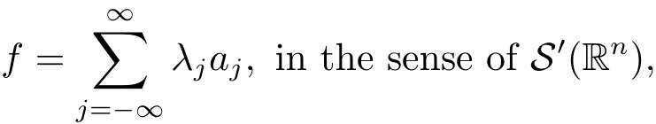
where ajis a central(α,p(·),s;)-atom with support contained in Bj,λj∈ R and

Moreover,

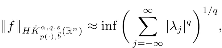
where the in fimum is taken over all above decompositions of f.

Our main result in this section can be stated as follows.

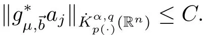
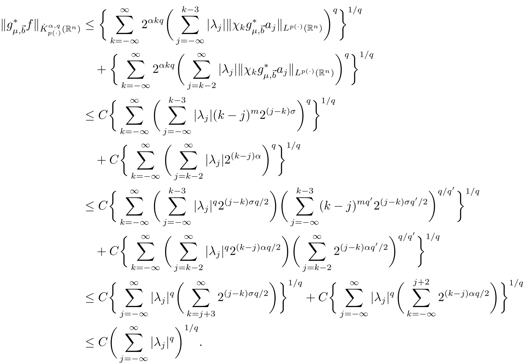
Theorem 4.1 Suppose 0＜ γ ＜ 1 and µ ＞ 3+2/n+2γ/n.If p(·)∈ P(Rn)TLH(Rn),0 ＜ q＜ ∞ and nδ2≤ α ＜ nδ2+γ,where δ2is the constant appearing in Lemma 2.2.Then the multilinear commutatorsmapinto

Proof Let ajbe a central(α,p(·),0;→b)-atom with support contained in Bj.We first restrict 0＜q≤1.In this case,it suffices to show that

We write

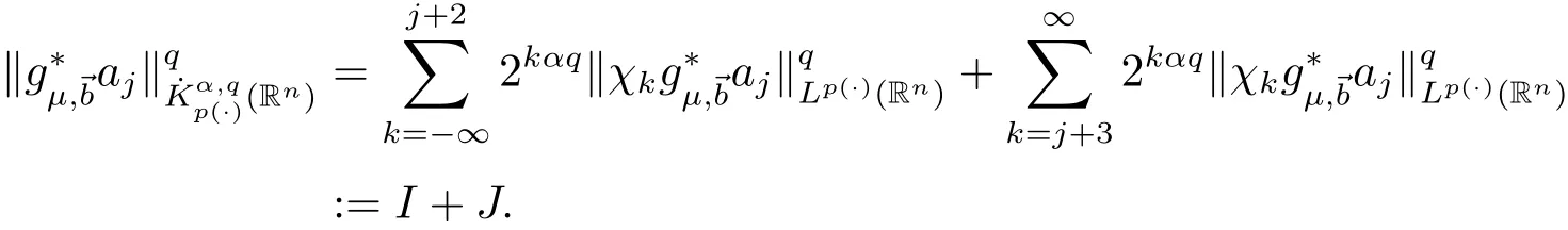
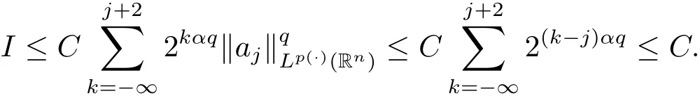
For I,by the boundedness ofin Lp(·)(Rn),we obtain

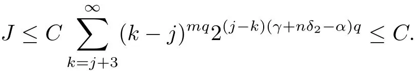
We proceed now to estimate J.If x∈Rk,y∈Bjand k≥j+3,then 2|y|＜|x|.By the vanishing condition of aj,we get that

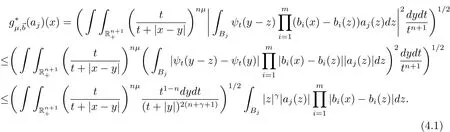
Ifµ ＞ 3+2/n+2γ/n,using the same estimates in[3,page 5],then we have

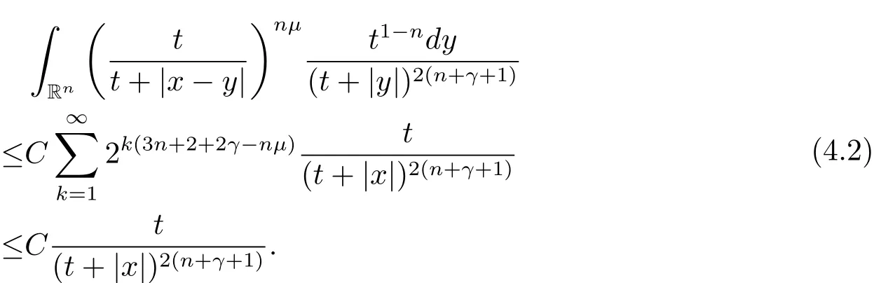
Combining(4.1)and(4.2),we arrive at the estimate

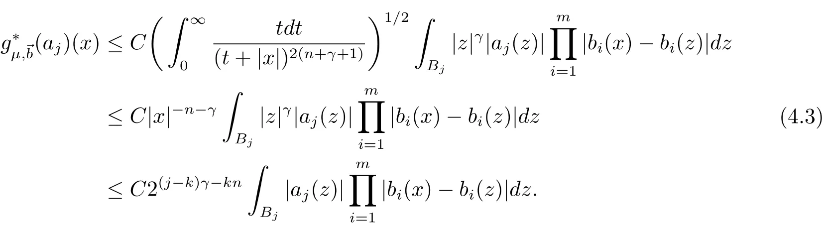
Let λi=(bi)Bj.An application of(4.3),(2.1),Lemmas 2.5,2.1 and 2.2 give

Consequently,by the condition γ +nδ2− α ＞ 0,we have

This completes the proof of Theorem 4.1.