HU Gui-kai,XIONG Peng-fei,WANG Tong-xin

(School of Science,East China University of Technology,Nanchang 330013,China)

Abstract:In this paper,we investigate the prediction in a finite population with the normal inverse-Gamma prior under the squared error loss.First,we obtain Bayes prediction of linear quantities and quadratic quantities based on Bayesian theory,respectively.Second,we compare Bayes prediction with the best linear unbiased prediction of linear quantities according to statistical decision theory,which shows that Bayes prediction is better than the best linear unbiased prediction.

Keywords: Bayes prediction;linear quantities;quadratic quantities; finite populations

1 Introduction

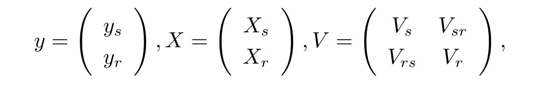
LetP={1,···,N}denote a finite population of N identifiable units,where N is known.Associated with the ith unit ofP,there are p+1 quantities:yi,xi1,···,xip,where all but yiare known,i=1,···,N.Let y=(y1,···,yN)′and X=(X1,···,XN)′,where Xi=(xi1,···,xip)′,i=1,···,N.Relating the two sets of variables,we consider the linear model

where β is a p× 1 unknown parameter vector,V is a known symmetric positive definite matrix,but the parameter σ2＞ 0 is unknown.

For the superpopulation model(1.1),it is interesting to study the optimal prediction of the population quantity θ(y)such as the population Total,the population variance,where=T/N is the population mean and the finite population regression coefficient βN=(X′V−1X)−1X′V−1y,and so on.In the literature,a lot of predictions for the population quantities were produced.For example,Bolfarine and Rodrigues[1]gave the simple projection predictor,and obtained necessary and sufficient conditions for it to be optimal.Bolfarine et al.[2]studied the best unbiased prediction of finite population regression coefficient under the generalized prediction mean squared error in different kinds of models.Xu et al.[3]obtained a kind of optimal prediction of linear predictable function,and got the necessary and sufficient conditions for any linear prediction to be optimal under matrix loss.Xu and Yu[4]further gave the admissible prediction in superpopulation models with random regression coefficients under matrix loss function.Hu and Peng[5]obtained some conditions for linear prediction to be admissible in superpopulation models with and without the assumption that the underlying distribution is normal,respectively.Furthermore,Hu et al.[6–7]discussed the linear minimax prediction in the multivariate normal populations and Gauss-Markov populations,respectively.Their results showed that linear minimax prediction for finite population regression coefficient is admissible in some conditions.Bolfarine and Zacks[8]studied Bayes and minimax prediction under square error loss function in a finite population with single parametric prior.Meanwhile,Bansal and Aggarwal[9–11]considered Bayes prediction of finite population regression coefficient using a balanced loss function under the same prior information.There are two characteristics in the above studies.

On the one hand,they obtained the optimal,linear admissible and minimax predictions based on statistical decision theory.It is well known that statistical decision theory only consider the sample information and loss function and do not consider the prior information.However,people usually have these information.

On the other hand,they discussed the Bayes prediction by considering the prior information of single parameter,and did not consider the situation of multi-parameters.In other words,they only made use of the prior information of regression coefficient,but not use the prior information of error variance in model(1.1).In fact,multi-parameter situations are often encountered in the practical problems.Therefore,in this paper,we will study Bayes prediction of linear and quadratic quantities in a finite population where regression coefficient and error variance have the normal inverse-Gamma prior.

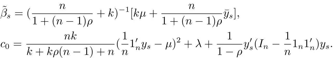
Assume that the prior distribution of β and σ2is normal inverse-Gamma distribution,that is,

whereµ is a known p×1 vector,α and λ are known constants,k−1is a ratio between the prior variance of β and sample variance of model(1.1).We can suppose that k−1is known by experience or professional knowledge.Therefore,the joint prior distribution of(β,σ2)is

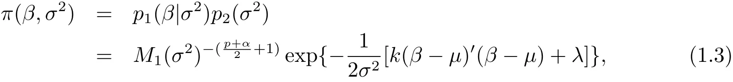
where X and Xsare known column full rank matrices.

The rest of this paper is organized as follows:in Section 2,we give Bayes predictor of population quantities in the Bayes model(1.4).Section 3 is devoted to discuss Bayesian prediction of linear quantities.In Section 4,we obtain Bayes prediction of quadratic quantities.Some examples are given in Section 5.Concluding remarks are placed in Section 6.

2 Bayes Prediction of Population Quantities

In this section,we will discuss the Bayes prediction of population quantities.Letbe a loss function for predicting θ(y)by.The corresponding Bayes prediction risk ofin model(1.4)is defined aswhere the expectation operator Eyis performed with respect to the joint distribution of y and(β,σ2).The Bayes predictor is the one minimizing the Bayes prediction riskIn particular,when we consider the squared error loss,then the Bayes prediciton of θ(y)is

and the Bayes prediction risk is

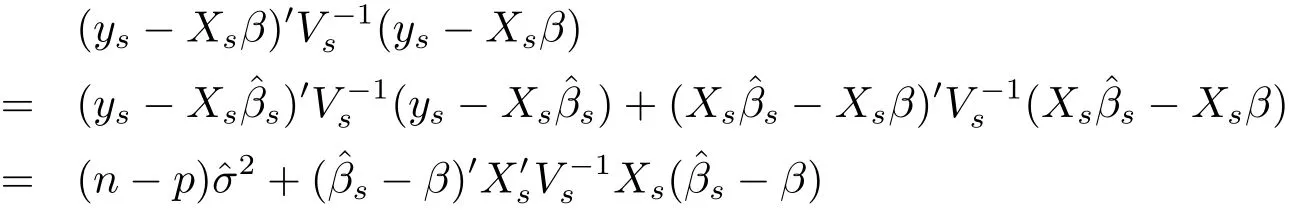
where the expectation operator Eysis performed with respect to the joint distribution of ysand(β,σ2).It is noted that ys|β,σ2∼ Nn(Xsβ,σ2Vs)and

This together with eq.(1.3)will yield the following results.

Theorem 2.1 Under the Bayes model(1.4),the following results hold.

(i)The joint posterior probability density of(β,σ2)is

(ii)The marginal posterior distribution of β is p-dimensional t distributionwith probability density

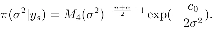
(iii)The marginal posterior distribution of σ2iswith probability density

(iv)Bayes prediction distribution of yrgiven ysis N−n dimensional t distributionwith probability density

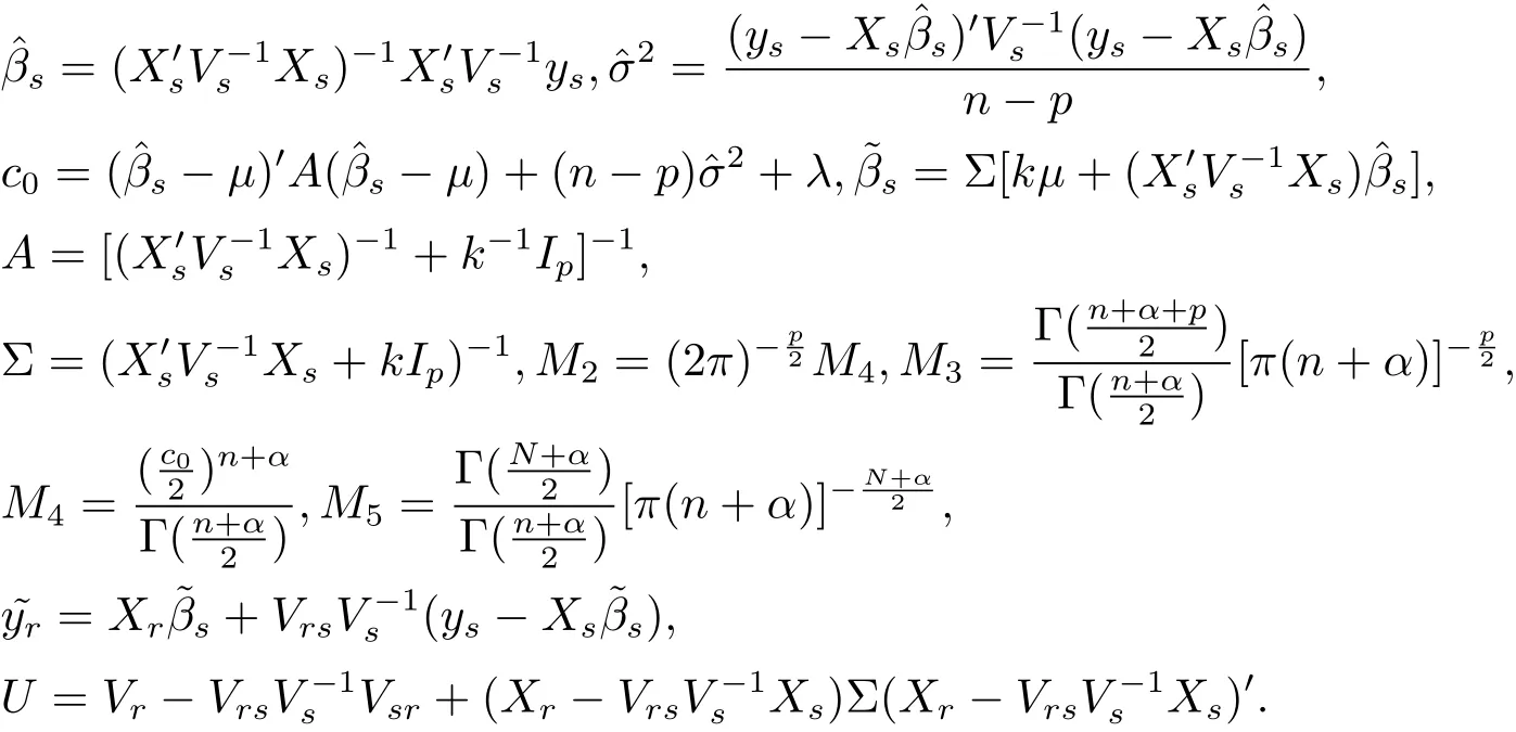
where

Proof The proof of(i):since

and ys|β,σ2∼ Nn(Xsβ,σ2Vs),the conditional probability density of ysgiven(β,σ2)is

This together with eq.(1.3)will yield that the joint posterior probability density of(β,σ2)is

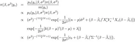
where m(ys)is the marginal probability density of ys,symbol∝denotes proportional to.By adding the regularization constantto eq.(2.3),we obtain result(i).

The proof of(ii):by the integral of eq.(2.2)about σ2,we have

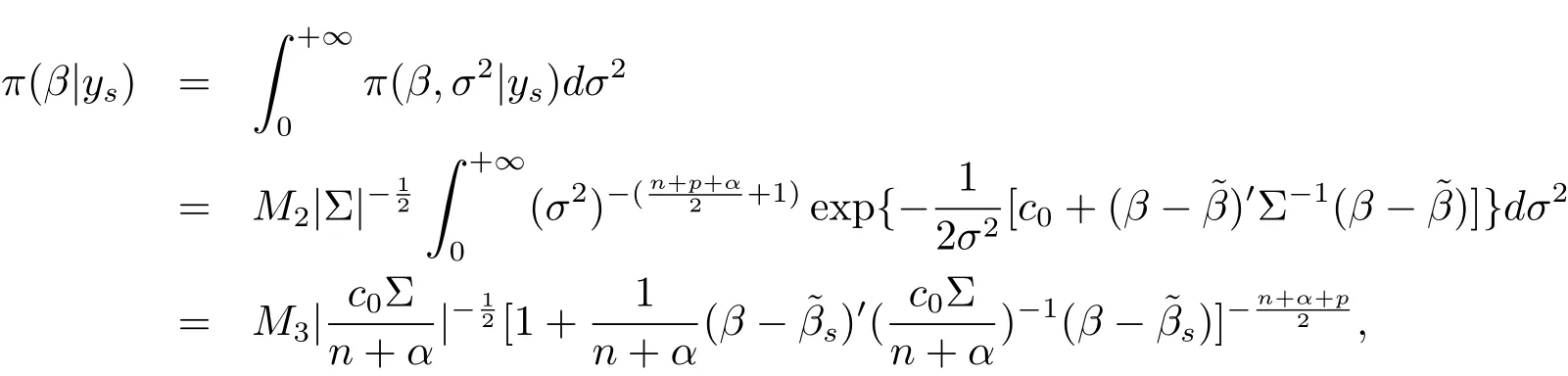
which implies that the marginal posterior distribution of β is p-dimensional t distribution with mean vector,correlation matrixand degrees of freedom n+α.

The proof of(iii):by the integral of eq.(2.2)about β,we can obtain the result.Here it is omitted.

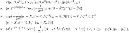
where

Adding the regularization constant to eq.(2.3)and integrating it by β and σ2,respectively,we can obtain the result.

3 Bayes Prediction of Linear Quantities

In order to obtain Bayes prediction of θ(y),we consider the squared error loss

then Bayes prediciton of θ(y)is

and Bayes prediction risk is

where the expectation operator Eysis performed with respect to the joint distribution of ysand(β,σ2).By result(iv)of Theorem 2.1,we know

and

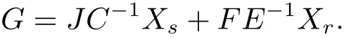
Now,let θ(y)=Qy be any linear quantity,whereis a known 1 × N vector.According to Theorem 2.1,eqs.(3.4)and(3.5),we have the following conclusions.

Theorem 3.1 Under model(1.4)and squared error loss function,Bayes predictor of linear quantity Qy is,and Bayes predictor risk is

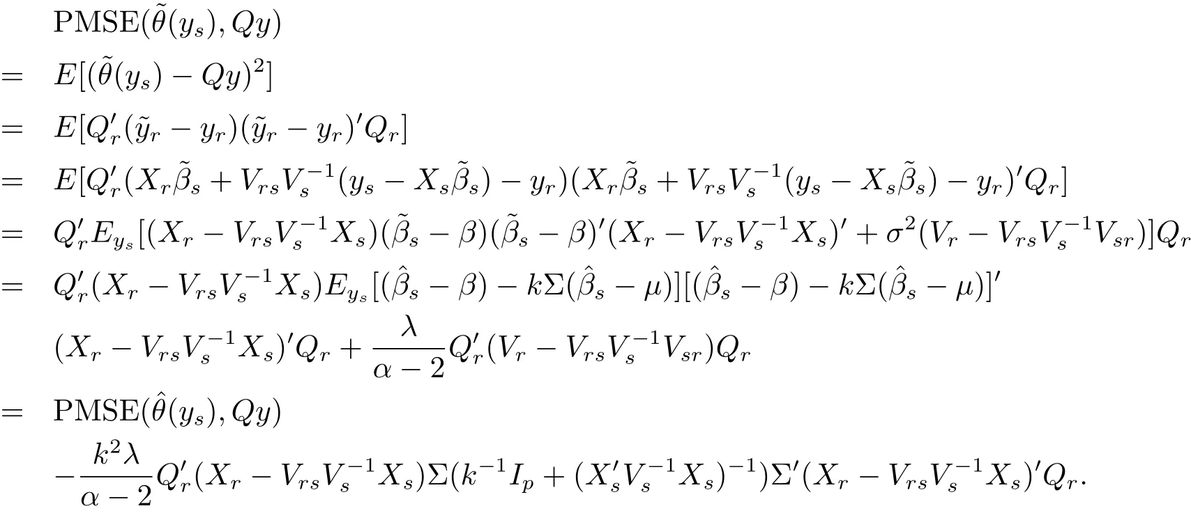
As we know,the best linear unbiased prediction of Qy under the squared error loss is,where,and.In the following,we will discuss the superiority between Bayes prediction and the best linear unbiased prediction under the predicative mean squared error(PMSE),which is defined by PMSE(d(ys),Qy)=E[(d(ys)−Qy)2].

Theorem 3.2 Under model(1.4),Bayes predictionof Qy is better than the best linear unbiased predictionunder the predicative mean squared error.

Proof By the definition of PMSE and,we have

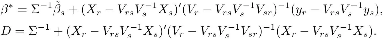
Corollary 3.1 Bayes predictor of the population total T under model(1.4)and the loss function(3.1)isand Bayes risk of this predictor isMoreover,is dominated byunder the predicative mean squared error,where

For the finite population regression coefficientfollowing Bolfarine et al.[2],we can write it as

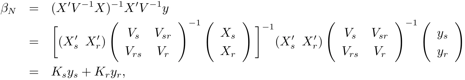
where

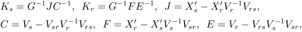
and

Then by Theorem 3.1,we have the following corollary.

Corollary 3.2 Bayes predictor of the population total βNunder model(1.4)and the loss function(3.1)isand Bayes risk of this predictor is.Moreover,it is better thanunder the predicative mean squared error,where

In order to illustrate our results,we give the following example.

Example 3.1 Let X=(x1,x2,···,xN)′,V=diag(x1,x2,···,xN)in the Bayesian model(1.4),where xi≠0,i=1,2,···,N.If Xs=(x1,x2,···,xn)′,ys=(y1,y2,···,yn)′,we haveAccording to Theorem 3.1,we have the following conclusions.

In the following,we continue to give the simulation study to explain our results according to the following steps,which are executed on a personal computer using Version 7.9(R2009b)Matlab software.

(i)Generating randomly a N×p full column rank matrix X and a p-dimensional vectorµ;

(ii)The number σ2and random error ε are generated from distributionand N(0,σ2V),respectively;

(iii)Generating a p-dimensional vector β by the distribution

(iv)Obtaining the dependent variable y by the model y=Xβ+ε.

(v)Generating randomly N-dimensional vector Q,then Bayes prediction and the best linear unbiased prediction of Qy are derived by Theorem 3.1,respectively.

(vi)Finally,we compare the PMSE between Bayes prediction and best linear unbiased prediction.

Now,we assume that N=10,n=6,p=3,α =8,λ =12,k=10,and obtain the above data.The simulation study shows that Bayes prediction is better than the best linear unbiased prediction,which is consistent to our theoretical conclusions.Here,we give the above data in one experiment as following.

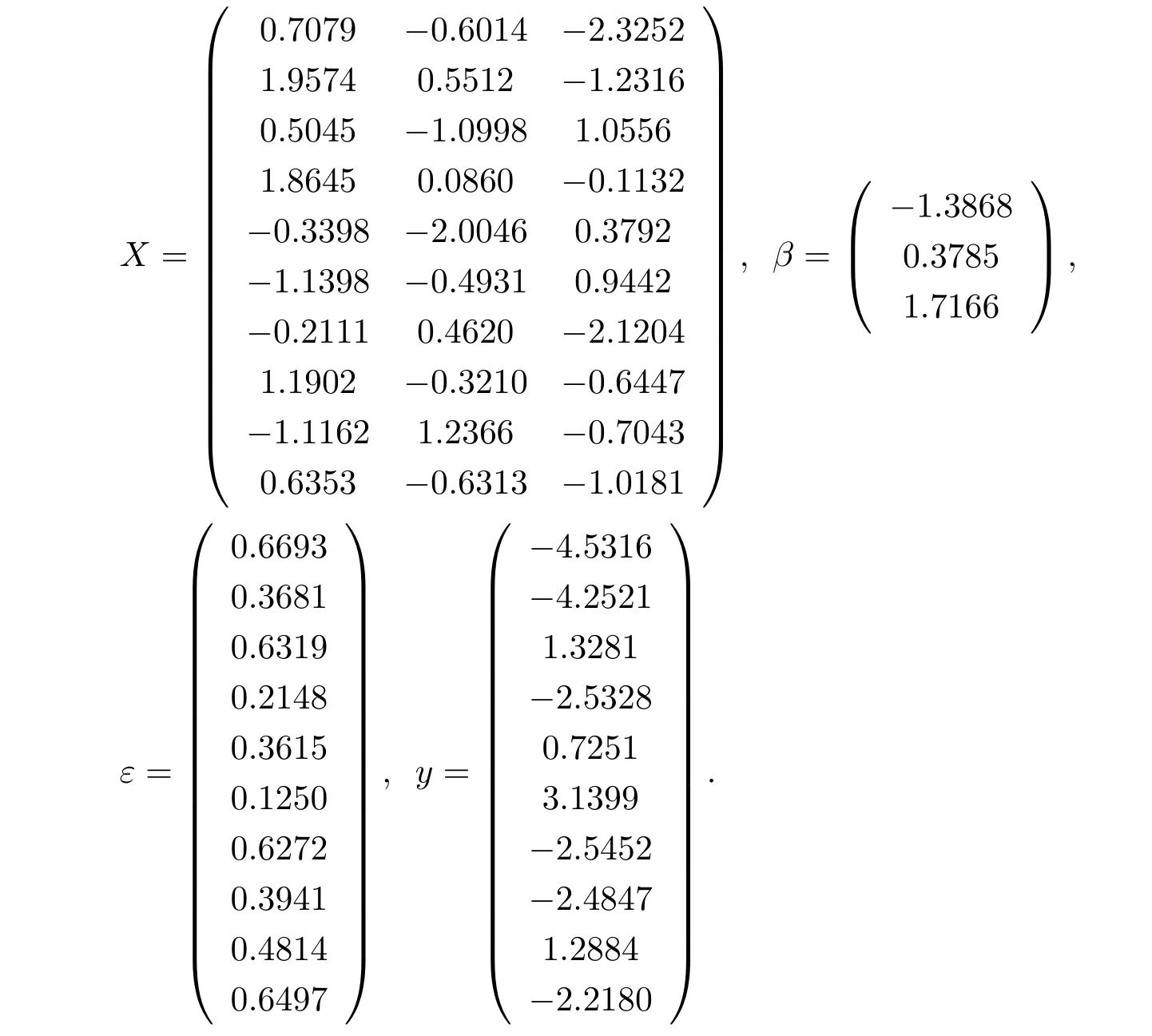
At this time,we get randomly

By direct computation,we have Qy=−4.3971.By Theorem 2.1,we know−4.8497,=−5.7928,andTherefore,Bayes prediction of Qy is better than the best linear unbiased predictor.

4 Bayes Prediction of Quadratic Quantities

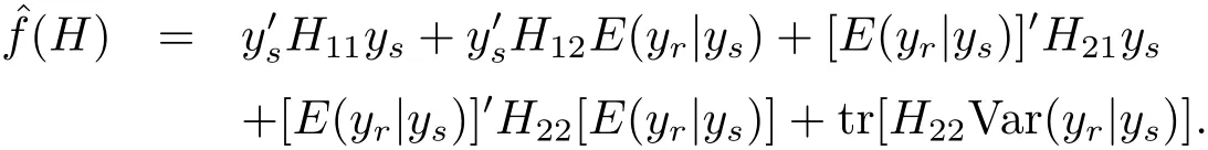
In this section,we will discuss Bayes prediction of quadratic quantities f(H)=y′Hy,where H is a known symmetric matrix.Assume thatwith H12=then

By Theorem 2.1 and eq.(3.2),we have the following results.

Theorem 4.1 Under model(1.4)and the loss function(1.3),the Bayes prediction of f(H)is

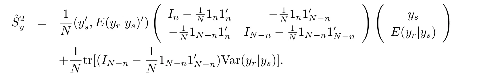
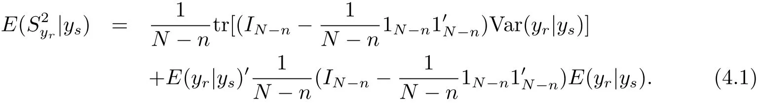
For the population variance,we know that

where 1ndenotes n dimensional vector with elements 1.Then by Theorem 4.1,we can obtain the following corollary.

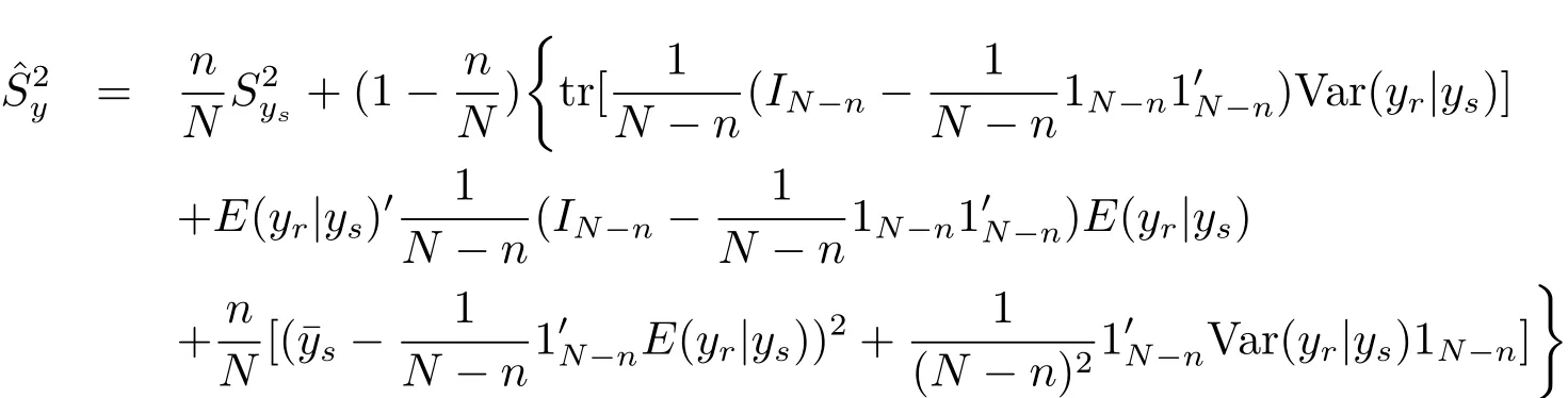
Corollary 4.1 The Bayes prediction of the population varianceunder model(1.4)and the loss function(3.1)is

Remark 4.1 The Bayes prediction of the population varianceunder model(1.4)and the loss function(3.1)is

According to eqs.(4.1)–(4.2)and the expression of,we can derive the result of this remark.It is easy to verify that the result of this remark is consistent to Corollary 4.1.

Then,

5 Concluding Remarks

In this paper,we obtain Bayes prediction of linear and quadratic quantities in the finite population with normal inverse-Gamma prior information.In our studies,on the one hand,the distribution of the superpopulation model is need to be normal.However,in many occasions,the distribution of the model is usually unknown in addition to the mean vector and covariance matrix.At this time,how to deal with the Bayes prediction?On the other hand,if the prior distribution is hierarchical and improper,how to obtain the generalized Bayes prediction and discuss its optimal properties?Such as these problems are deserved to discuss in the future.