Tenglong Su ,Fengling Yang ,2,*,Meiting Li ,Kanghui Wu

1 School of Mechanical Engineering,Shandong University,Jinan 250061,China

2 Key Laboratory of High Efficiency and Clean Mechanical Manufacture(Shandong University),Ministry of Education,Shandong University,Jinan 250061,China

Keywords:Covering-plate Rushton impeller(RT-C)Power consumption Flow pattern Mean velocity Mixing time Computational fluid dynamics(CFD)

A B S T R A C T A modified Rushton impeller with two circular covering-plates mounted on the upper and lower sides of the blades was designed.There are gaps between the plates and the blades.The turbulent hydrodynamics was analyzed by the computational fluid dynamics(CFD)method.Firstly,the reliability of the numerical model and simulation method was verified by comparing with the experimental results from literature.Subsequently,the power consumption, flow pattern,mean velocity and mixing time of the covering-plate Rushton impeller(RT-C)were studied and compared with the standard Rushton impeller(RT)operated under the same conditions.Results show that the power consumption can be decreased about 18%.Compared with the almost unchanged flow field in the lower stirred tank,the mean velocity was increased at the upper half of the stirred tank.And in the impeller region,the mean axial and radial velocities were increased,the mean tangential velocity was decreased.In addition,the average mixing time of RT-C was shortened about 4.14%than the counterpart of RT.The conclusions obtained here indicated that RT-Chas a more effective mixing performance and it can be used as an alternative of RT in the process industries.

1.Introduction

Although the rudiment of agitation can be traced back to 1556,systematic studies only started in the 1950s,and the first international conference on mixing in the industrial processes was held in 1963[1,2].Ever since the beginning,exploring of the flow and mixing behavior of fluids in stirred tanks has always been the center of attention among chemical engineers and scientific researchers.To date,we can say that the basic phenomena and mechanisms of fluid mixing,especially the single-phase flow,have been clarified to a certain degree of maturity.Notwithstanding,intensification of mixing efficiency has always been one of the everlasting research topics.

During the past several decades,great efforts have been devoted to enhance the fluid mixing in stirred tanks,among which considerable attention has been paid to the impeller.These can be roughly classified into the following four categories.The first is optimization of impeller size,location and configuration,which have profound impacts on the flow fields and in turn govern the mixing efficiency.Take the standard Rushton impeller as an example,the impeller-to-tank diameter ratio,D/T,is typically between 1/4 and 1/2 with the standard ratio being 1/3.The off-bottom clearance is usually C=T/3.The length and width of the blade are l=D/4 and w=D/5,respectively[3].For the single-impeller stirred tank,the off-bottom clearance determines the flow pattern[4–7].For the multiple-impeller stirred tank,the impeller spacing is another dominant parameter[8].Developing new types of impellers is the second work.For instance,Smith[9]designed the reversible mixing impeller for the chemical processing industry.It generates an axial flow when it rotates in one direction and a radial flow when it rotates in the opposite direction.Bakker and Ohio[10]proposed the Scaba impeller.It has vertically asymmetric concave blades.This and subsequent studies show that this impeller has a flatter gassed power curve and can disperse more gasbefore flooding than the impellers with symmetric blades[11,12].Liu et al.[13]developed the rigid– flexible combination impeller.They studied the liquid–liquid mixing of two immiscible fluids in a laboratory-scale mixer–settler and enhancement of mixing ability was experimentally observed.The third is the employment of draft tube,which is vertically mounted around the impeller and shaft at the desired axial location.The draft tube may have different configurations,such as conical shape and cylindrical shape.Use of draft tube can enhance the axial flow capacity,and accordingly increase the mixing efficiency and mass transfer performance.At the same time,the power consumption also increases[14–20].How ever,there is divergent opinion.Houcine et al.[21]pointed out that the use of draft tube with the rounded or profiled tank bottom may significantly reduce the power consumption,while the mixing time is much larger.The final is the application of chaotic mixing theory in the fluids mixing in stirred tanks[22].These can be divided into two categories:spatial chaotic mixing and temporal chaotic mixing[23].Spatial chaotic mixing involves altering on the mounting position and motion form of the impeller.The pioneering works in this area are eccentric agitation[24],inclined-shaft agitation[25],side-entering agitation[26],reciprocating agitation[27],and so on.Temporal chaotic mixing mainly refers to the unsteady stirring approaches,which include co-reverse periodic rotation and time-periodic fluctuation of impeller rotational speed[28,29].These studies indicate that chaotic mixing has a potential for dramatic improvement of performance of chemical processes,especially for those operated under the laminar flow regime.And it is recognized that“the only efficient route to mix in laminar flow s is by chaos”[30].

In terms of the Rushton impeller,it has been wildly used in the chemical,pharmaceutical,biochemical and other industrial operations.And some impellers were designed based on the traditional Rushton impeller.Yang et al.[31]investigated the dislocated-blade Rushton impeller in gas–liquid mixing in a baffled stirred vessel using the experimental and CFD methods.Liu et al.[32]designed the rigid– flexible coupling impeller and punched- flexible impeller by adding flexible blades and punning on the RT.Yang et al.[33]proposed a novel six-blade grid disc impeller(RT-G)and the single-phase turbulent flow and mixing in a baffled stirred tank agitated by this impeller were numerically studied by the detached eddy simulation(DES)model.

The present work was prompted by the need for improving the mixing efficiency of fluids in stirred tanks.As an alternative to the standard Rushton impeller,the covering-plate Rushton impeller was proposed.The turbulent hydrodynamics of the liquid phase flow and mixing in the stirred tank agitated with this impeller were studied.The results were compared with the standard Rushton impeller to validate its merits.

2.Stirring System

Schematic diagrams of the stirring system investigated here are given in Fig.1.To compare with the literature results,it has the same configurations and dimensions as that studied by Wu et al.[34].The cylindrical tank has an inner diameter of T=0.27 m.Two kinds of impellers,the standard Rushton impeller and the covering-plate Rushton impeller(hereinafter referred to as RT and RT-C,respectively)proposed by the authors,were employed in the study.The diameter of the two impellers is D=0.093 m and the impeller was located with the off-bottom clearance of C=T/3.The length and width of impeller blade are l=D/4 and w=D/5 respectively.Diameter of the impeller disc is 0.07 m.The thicknesses of the blades and the circular covering plate are 2 mm.The inner diameter and outer diameter of the covering plate are 0.047 m and 0.093 m respectively and the gaps between blades and plates are 4 mm.The assembly relationship between the two covering-plates and the Rushton impeller are as shown in Fig.1(d).The plates can be made of light materials like plexiglass or UHMW-PE so as to reduce the mass.Four full height baffles with the width of B=0.027 m were evenly mounted around the tank wall and the first baffle was positioned at the angle position ofθ=0°.Purewater with the density of ρl=998.2kg ·m−3and the dynamic viscosity of μl=0.001Pa ·s was used as the working fluid.The height of the liquid level was H=0.27 m.The impeller rotated in the anticlockwise direction with the speed of N=200 r·min−1.The corresponding impeller tip speed was Utip= πND/60=0.973m ·s−1.The Reynolds number was Re= ρND2/μl=2.87×104.

Fig.1.Configuration of the stirring system:(a)stirred tank:1-stirred tank,2-baffle,3-strring shaft,4-impeller,(b)top view of the stirred tank,(c)RT,(d)RT-C.

3.Numerical Simulation

3.1.Numerical models

The turbulent fluid flow in the stirred tank was predicted by the standard k-ε model,which is a semi-empirical formula mainly based on the turbulent kinetic energy and the turbulent dissipation rate.The governing equations of this model can be given as follow s:

The non-reacting mixing process was modeled so as to obtain the mixing time.The transient scalar transport equation(Eq.(3))was solved to follow the dynamic distribution of the scalar tracer:

This equation assumes that the tracer is distributed in the stirred tank by convection and diffusion[35].Here,c is the tracer volume fraction,u is the velocity vector,Dmis the molecular diffusivity of the scalar,μtis the turbulent viscosity and σtis the turbulent Schmidt number it was taken as 0.7 in the present study.For the meanings of the other parameters,one may refer to the section “Nomenclature”.

3.2.Computational grid

Considering the instability of the flow,the whole stirred tank was simulated.The rotation of the impeller was simulated using the sliding mesh method.In this study,the tank was divided into two regions,one rotor and one stator.The rotor consists of the impeller and its adjacent regions and the stator encompasses the rest of the tank.When constructing the geometry model,the origin of coordinate system coincides with the center of the stirred tank bottom.The radial boundary of the rotor region was at r=0.07 m.And the axial boundaries of the rotor region were positioned at 0.06＜z＜0.12(where z and rare the axial and radial coordinates,respectively).

The grid was prepared with the preprocessor ICEM CFD 16.0 and the grid independence had been studied before the final grid nodes were determined.The computational domain was discretized using a uniformly distributed hexahedron structured mesh consisting of approximate 1285000 nodes.Ranade et al.[36]and Ng et al.[37]reported that at least 200 grid nodes are required to resolve the blade surface so as to capture details of the flow near the impeller.Derksen et al.[38]also pointed out that no less than 8 grid nodes are required along the impeller blade width so as to model the mean flow field correctly.According to these guidelines,we used r×θ×z:24×2×18 grid nodes.There are 5472 grid nodes on the surface of the covering-plate and 3 grid nodes in thickness direction of the covering-plate.The quality of mesh was evaluated using the Pre-mesh quality criterion.The minimum value of the volume mesh was 0.75,which indicates that the mesh is acceptable.

3.3.Initial and boundary conditions

The initial velocity of the liquid in the stirred tank was assumed to be zero.The tank walls,baffles and impeller were treated as non-slip boundaries with standard wall functions.A rotation wall boundary condition was set for the shaft.The interfaces between rotor and stator were set as the interface boundary condition.At the top of the computational regime,the symmetry boundary condition was applied.

3.4.Modeling approach

The transient pressure-based Navier–Stokes algorithm was used for the solution of the model with implicit double precision solver formulation where the absolute velocity formulation was adopted.The SIMPLE algorithm was used for pressure–velocity coupling.Time-marching was used by a fully-implicit first order scheme.The second order upwind scheme was adopted for spatial discretization of the momentum,turbulent kinetic energy and turbulent dissipation rate equations.Based on the current mesh topology,the time step was set at 0.02 s and the Courant number was restricted less than 2.The time of numerical simulation was 18 s.The solution was considered to be fully converged when the normalized residuals of all variables were less than 1×10−4.All the simulations were carried out using the ANSYS Fluent 16.0(Fluent Inc.,USA)on a Window s-x64 In spur NP5540M3 server with thirty-two Intel Xeon E5-2440 v2(1.90 Hz)processors and 16 GB DDR3 RAM in a parallel model.

4.Results and Discussion

4.1.Simulation method verification

The fluid flow in the impeller region is very complicated,so it is persuasive to choose the mean velocities around the impeller to compare with the experimental result of the literature[34]to verify the numerical model and the simulation method.All the velocities are extracted at the radial position of r=70 mm,located within the axial[2(z-C)/w]height range of−2 to 2.The profiles of the mean axial velocity Uz,radial velocity Urand tangential velocity UΘnormalized by the impeller tip velocity Utipare shown in Fig.2.We can see that the variation trend of each mean velocity is identical.Generally speaking,the numerical results agree well with the experiment data.

Fig.2.Comparisons the profiles of the mean(a)axial,(b)radial and(c)tangential velocity generated by simulation and experiment.

4.2.Power consumption

Power consumption is a very important parameter which contributes significantly to the overall operation cost of the stirred tank.The methods of measuring power consumption can be divided into two categories,experimental method and numerical simulation method.Many experimental devices can be used to measure power consumption in stirred tanks,and these were reviewed by Ascanio et al.[39].In the present work,we used the computational numerical simulation technology to simulate the stirring process.The numerical value of stirring torque M can be extracted from simulation results.Usually,power consumption can be expressed as the dimensionless power number:

where P is the power consumption:

The procedure of calculating power estimation directly from the total torque required to rotate the shaft and impeller is reliable because of the fact that the flow field around the impeller is resolved.To reduce the computational time requirement,it is not necessary to calculate the viscous energy dissipation term from the calculated velocity field[40].

The torques and power numbers of RT and RT-C are shown in Table 1.The simulated power numbers of RT and RT-C were 4.967 and 4.072,respectively.From a quantitative comparison,we can easily find the power number of RT-C was lower than the power number of RT,about 18%decreased.For RT operated in the fully turbulent flow regime,the power number is about 5.4[8,11].In terms of the numerical result obtained here,it is approximately 8%under-predicted.This may be attributed to the weakness of the standard k=ε model.So we think the numerical results of RT and RT-C are credible,the RT-C is highlighted in reducing power consumption than RT.

Table 1Torque and power number of RT and RT-C

4.3.Flow field

Flow field is affected by many factors,such as types of impeller and tank geometry,number of blades,liquid height and fluid properties.The flow field of a stirred tank contains lots of information that can be used to demonstrate the mixing performance,such as flow pattern,velocity distribution and turbulent kinetic energy.In this section,we compare the flow pattern and the mean velocities generated by RT and RT-C.

4.3.1.Flow pattern

Flow pattern shows the types of fluid circulation in the stirred tank.Radial flow,axial flow and tangential flow are the three common flow patterns,also they exist in a flow field at the same time.Here,the transient flow fields were simulated.We chose the velocity vector at the time instant t=6 s(the flow field is already relatively stable)in the θ =0°plane as an example to demonstrate the differences of flow structure between RT and RT-C.The results are shown in Fig.3.

According to the reported researches about the standard Rushton impeller,we know that its flow pattern is radial flow.From an overall perspective,the simulated flow fields of RT and RT-C are consistent with this characteristic.The large circulation loops,irregular secondary recirculation structures and many small vortexes of different scales are present in the bulk of the stirred tank.How ever,there are two obvious differences of the velocity vector generated by these two impellers.The most conspicuous difference is that the axial flow capacity generated by RT-C is improved.From Fig.3,we can see that the velocity of RT-C is larger than RT at the upper part of the stirred tank.So,RT-C could promote the velocity far away from the impeller effectively.Furthermore,it is apparent that the velocity vector generated by RT-C presents radiation shape around impeller while the velocity vector generated by RT is radial.It means the flow field in the vicinity of RT-C can reach a high turbulent flow in a shorter time.Through above analysis,we can find that RT-C has significant impact on improving the uniformity of velocity in the stirred tank.The differences among other parameters will be discussed in the following content.

Fig.3.Velocity vectors of(a)RT and(b)RT-C in the θ =0°plane at the time t=6 s.

4.3.2.Mean velocity profile

Fig.4.Comparisons between the axial profiles of the mean(a)axial,(b)radial and(c)tangential velocity generated by RT and RT-C.

Fig.4(continued).

Profiles of the mean axial,radial and tangential velocity in the vertical plane θ =0°of the stirred tank are shown in Fig.4.In these plots,the mean velocities were normalized by the impeller blade tip velocity Utipand the axial height z was normalized by the blade width.Overall,the mean velocity distribution tendency of RT and RT-C is consistent.For example,in terms of the radial and tangential velocity,the velocity decreases from the center-line of the blades.How ever,the velocity magnitude is different,especially at r=5.0 cm.It is apparent that the mean axial velocity of RT-C is larger(in the range of−0.14 to 0.17)than that of RT,which is−0.06 to 0.10.The mean radial velocity of RT-C increases at r=5.0 cm,especially at the axial height of 2(z−C)/w=0 with the maximum increase of 17%.From the first plot of Fig.4(b)and(c),because of the two covering-plates on the upper and lower sides of the blades,we can easily find that the jet-like pattern of the impeller stream is changed at 2(z−C)/w=±1.In terms of the mean tangential velocity at r=5.0 cm,it decreases except for the position of the two covering-plates.

Fig.4(a)shows the mean axial velocity at four different radial positions in the stirred tank,i.e.,r=5.0 cm,7.7 cm,9 cm and 10.5 cm.At r=5.0 cm,the velocity changes prominently compared with the other positions.At r=7.7 cm,9.0 cm and 10.5 cm,the mean axial velocity increases above 2(z−C)/w=0 and decreases below this axial height.The mean radial velocity is shown in Fig.4(b),the velocity increases at r=5.0 cm and r=10.5 cm.How ever,it decreases at r=7.7 cm and r=9.0 cm,which is not desired.The cause may be that the impeller discharge flow generated by RT-C has already split into two streams at the position of r＜7.7 cm,one flowing upward and the other flowing downward into the bottom of the tank.Generally speaking,the mean tangential velocity decreases at the four radial positions,and this is useful for mixing process.From the analysis above,it can be concluded that RT-C has three main advantages:increasing mean axial velocity,decreasing tangential velocity and enhancing the turbulent flow especially in the impeller region.Accordingly,we can deduce that RT-C can improve the mixing performance.This will be verified in the following section.

4.4.Mixing time

Mixing time is an important parameter used to characterize the mixing performance.It can be determined based on the tracer concentration variation curves using the conventional 95%ruler,which means that the time required for the tracer concentration to reach within±5%of the

final equilibrium value is the mixing time.Two tracer injection positions were set and four concentration monitoring locations were selected,as shown in Fig.5.The two tracer injection positions were denoted as T_1 and T_2.The former is below the top liquid surface and the latter is in the vicinity of blade.We can get the tracer concentration values from the numerical simulation results,based on which we can then obtain the tracer concentration variation curves.

Fig.5.Tracer injection(■)and concentration measurement locations(+)in theθ=0°plane.

Fig.6.Comparisons of the tracer concentration profiles between RT and RT-C at four measurement points generated by two different tracer injection locations.

The tracer concentration variation curves of the above-mentioned positions are shown in Fig.6.In these plots,the tracer concentration was normalized by the final fully mixed value.In each location,both RT and RT-C have large fluctuations of the tracer concentration,especially in the initial stage of mixing.Then,the tracer concentration reaches the fully mixed value and the mixing time is confirmed.The contour plots of the scalar concentration in the θ =0°plane,which clearly express the scalar concentration evolution in the stirred tank,are shown in Figs.7 and 8.The mixing time of RTand RT-C is given in Table 2.In terms of every monitoring point,the local mixing time is different due to the different tracer injection locations.Overall,the mixing time of RT-C is shorter than RT,except the point B at T_2.When the tracer injection location is at T_1,the mixing time of RT and RT-C is 10.03 s and 9.70 s,respectively.When the tracer injection location is at T_2,they are 9.50 sand 9.28 s.No matter the tracer was injected at T_1 or T_2,the mixing time of RT-C decreases when compared with RT.At T_1,the average mixing time of RT-C and RT is 9.70 and 10.30,with a decrease about 5.83%.At T_2,the decrease is 2.32%.The overall average mixing time of RT and RT-C is 9.90 s and 9.49 s,respectively.And the decrease is 4.14%.Therefore,we can conclude that RT-C is more efficient.When compared with RT,the stirred tank agitated with RT-C could reach the expected flow field faster.

Fig.7.Predicted tracer concentration distribution of RT as a function of time in θ =0°plane:(a)1 s,(b)3 s,(c)5 s and(d)7 s.

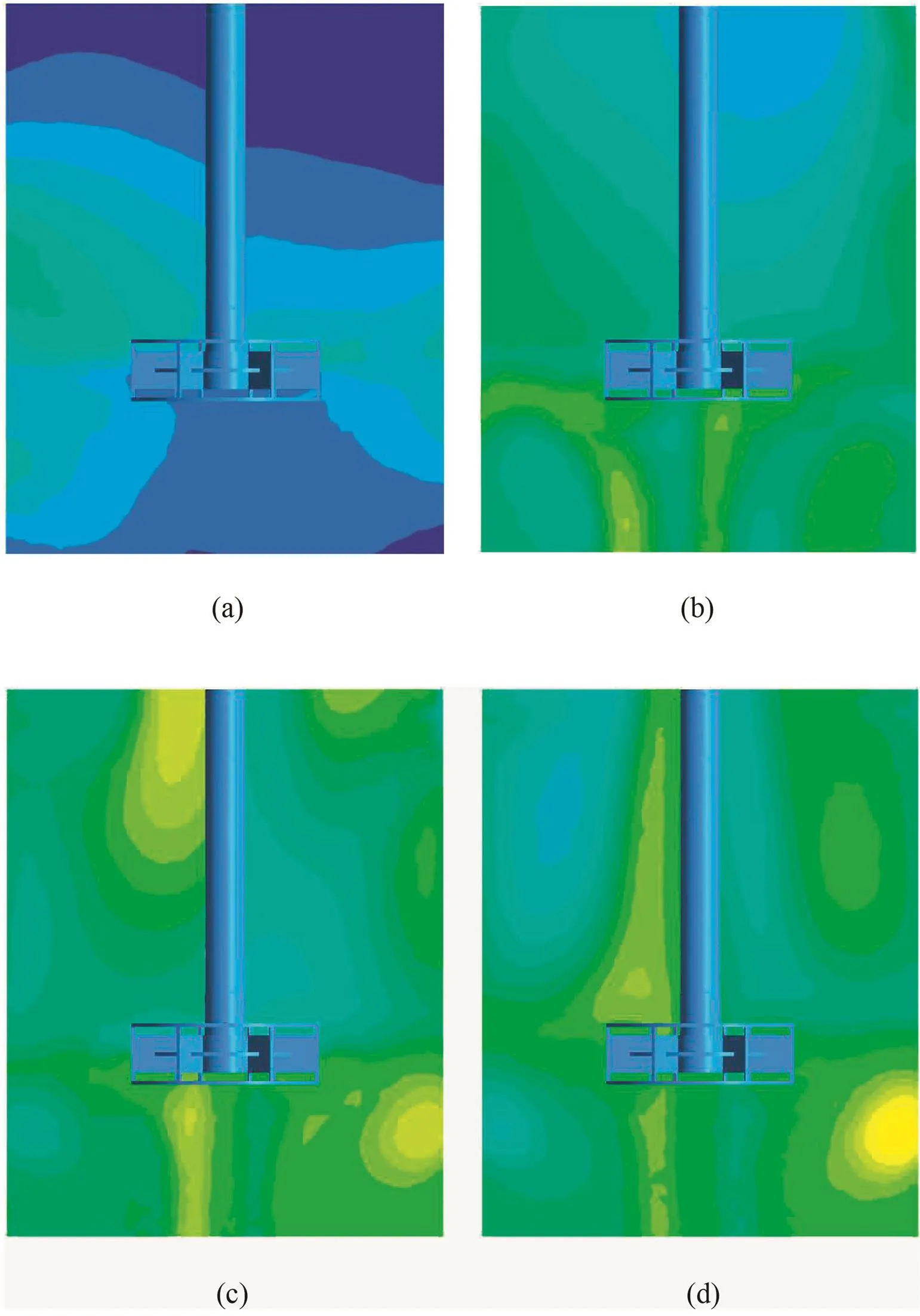
Fig.8.Predicted tracer concentration distribution of RT-C as a function of time in θ =0°plane:(a)1 s,(b)3 s,(c)5 s and(d)7 s.

Table 2Mixing time of RT and RT-C

5.Conclusions

Improving the mixing efficiency has always been,and still will be the research focus.In this paper,a kind of covering-plate Rushton impeller(RT-C),which is a modification of the standard Rushton impeller(RT),was designed.According to the above analysis,RT-C outperforms RT.The power consumption can be decreased about 18%.RT-C can alter the local flow pattern,the velocity vectors show that the flow field is more turbulent around the modified impeller.Also,the mean velocity can be increased in the vicinity of the impeller.In addition,the average mixing time of RT-C was shortened than RT,about 4.14%.Therefore,the impeller designed in this study has a promising application in the industrial processes.

Nomenclature

C impeller off-bottom clearance,m

Clεmodel constant,1.44

C2εmodel constant,0.09

c tracer volume fraction

D diameter of the impeller,m

Dmmolecular diffusivity,m2·s−1

Gkturbulent kinetic energy generation item,m2·s−3

H liquid height,m

k turbulent kinetic energy,m2·s−2

l blade length,m

M torque,N·m

N impeller rotation speed,r·min−1

Nppower number

n impeller rotation speed,r·s−1

p power,W

Re Reynolds number

r radial coordinate,m

T diameter of the stirred tank,m

t time,s

u velocity vector,m·s−1

Urmean radial velocity,m·s−1

Uzmean axial velocity,m·s−1

UΘmean tangential velocity,m·s−1

Utipimpeller tip speed,m·s−1

w blade width,m

z axial coordinate,m

ε turbulent dissipation rate,m2·s−3

θ tangential coordinate,(°)

μ dynamic viscosity,Pa·s

μtturbulent viscosity,Pa·s

ρ density,kg·m−3

σkturbulent Prandtl number,1.0

σtturbulent Schmidt number,0.7

σεturbulent Prandtl number,1.3