Bo Zhang,Lingtong Kong,Haibo Jin*,Guangxiang He,Suohe Yang,Xiaoyan Guo

Beijing Key Laboratory of Fuels Cleaning and Advanced Catalytic Emission Reduction Technology,Beijing Institute of Petrochemical Technology,Beijing 102617,China

Keywords:High-pressure bubble column Bubble coalescence Computational fluid dynamics Population balance model

A B S T R A C T In this study,based on the Luo bubble coalescence model,a model correction factor C e for pressures according to the literature experimental results was introduced in the bubble coalescence efficiency term.Then,a coupled modified population balance model(PBM)with computational fluid dynamics(CFD)was used to simulate a high-pressure bubble column.The simulation results with and without C e were compared with the experimental data.The modified CFD-PBM coupled model was used to investigate its applicability to broader experimental conditions.These results showed that the modified CFD-PBM coupled model can predict the hydrodynamic behaviors under various operating conditions.

1.Introduction

Bubble column reactor has simple structure,large capacity,easy operation,adequate heat and mass transfer,and small bed pressure drop[1–3].Therefore,bubble columns are widely used in industry including chemical engineering,petrochemical,bio-engineering,environmental energy etc.[4].Many scholars have applied the population balance model in studying atmospheric bubble columns[5–7].But bubble columns in chemical production are generally operated under high pressures and examples are hydrocracking of petroleum(P=5.0–21 MPa),Fischer-Tropsch synthesis(P=2.0–5.0 MPa)and benzene hydrogenation(P=5.0 MPa)[8–11].Although high-pressure bubble columns are widely used in chemical and biochemical processes,their fundamental hydrodynamic behaviors,which are essential for reactor scale-up and design,are still not fully understood.

The effect of pressure on the hydrodynamic behaviors of bubble columns has been experimentally investigated by many researchers.The gas holdup in high-pressure columns significantly increases due to the decreased bubble size[12–14].The gas–liquid mass transfer and reaction performance are enhanced as the pressure rises[10,15].With the development of computer technology,numerical simulation of gas–liquid two-phase flow has been greatly developed.Among them,Krishna et al.[16]used a CFD model to simulate the high-pressure bubble column with the drag force between gas and liquid was considered only,and a density correction term ρ/ρ0due to pressure change was introduced into the drag force model.Chen et al.[17]modified the gas density correction term in the drag model based on[16].Although the radial and axial velocity components were better predicted,the bubble diameter distribution was assumed constant.As the population balance model(PBM)can resolve the influence of bubble coalescence and breakup on bubble size distribution,the simulation of high-pressure bubble columns has been intensively conducted using the CFD-PBM coupled model in recent years.Wang et al.[18]imposed the energy and capillary constraints in the bubble breakup model,and got a modified PBM to express the effect of pressure.The bubble size distribution was then reasonably predicted by the modified PBM.Xing et al.[19]proposed a unified breakup model for both bubbles and droplets with the effect of pressure included.And this unified breakup model gave good predictions of both the effect of pressure(or gas density)on the bubble breakup rate and the different daughter size distributions of bubbles and droplets.Many works have been reported on the effect of pressure in bubble columns,but the mechanism of pressure effect was little addressed.

Although the influence of pressure on the hydrodynamics in bubble columns is pronounced and very important for the design and scale-up of reactors at high pressures,further studies need to be conducted on the effects of pressure.In this paper,based on the Luo bubble coalescence kernel model,a correction coefficient Ceabout density ρ/ρ0is introduced in the bubble coalescence efficiency item.The modified CFDPBM coupled model is used to simulate the flow field in a high-pressure bubble column.The effects of pressure on the gas–liquid two-phase flow in the high-pressure bubble column were investigated at 0.5–2.0 MPa.It is shown that the modified CFD-PBM coupled model can describe the effect of pressure on the hydrodynamic parameters in the high-pressure bubble column.

2.Mathematical Model

2.1.Two- fluid model

In the present work,the main approach for simulating gas–liquid flow s in a bubble column is Euler–Euler model.In contrast with the Euler–Lagrange approach,the gas phase and the liquid phase in the bubble column were considered as continuous phases of mutual penetration with the Euler–Euler approach.This approach gives a possibility of lower computational cost and particle size distributions.The control equations of the two- fluid model are generally based on the Reynolds-averaged method[20–22],assuming that the gas is incompressible,ignoring the heat transfer and mass transfer between the two phases.So a simplified form of control equations can be obtained:

Continuity equation:

Momentum conservation equation:

2.2.Turbulence equations

The standard k-ε model is selected for turbulence modeling.It is a classical representation of the Reynolds-averaged method.

The k and ε equations are:

with C1ε=1.44,C2ε=1.92,C3ε=1.2,Cμ=0.99,σk=1.0,σε=1.3.

Turbulent viscosity is calculated by:

2.3.Interphase forces

The exact expression of the interphase forces is the key to simulating the gas–liquid two-phase flows,and many researches exist on the inter phase forces between gas and liquid[23,24].In this work,the drag force,transverse lift force,turbulent dispersion force and wall lubrication force are considered.

2.3.1.The drag force

It is generally believed that the drag is the predominant force in modeling the gas–liquid flow s of bubble columns[25],as did in many simulation[14,26].Air bubbles are formed from the bottom of the tower with a certain gas velocity.In the control volume formulation,all bubbles in the control volume suffer the total drag force as follow s:

Liu et al.[23]introduced a modified drag coefficient CDin the bubble group drag model.And the modified drag model was used in the numerical investigations of the flow characteristics of pressurized churn turbulent bubble column with the operation pressure varying from 0.5 MPa to 2.0 MPa,and superficial gas velocity from 0.20 m·s−1to 0.31 m·s−1.The simulation results can accurately reflect varioushydrodynamic parameters in the bubble column.Therefore,their drag coefficient CD[23]is adopted in this work:

2.3.2.Turbulent dispersion force

In order to simulate the turbulence of the fluid in the high-pressure bubble column,it is necessary to introduce the turbulence diffusion force,which can help in making the gas holdup evenly distributed.A turbulent diffusion force formula proposed by Lopez de Bertodano[27]is as follows:

CTDisthe coefficient of turbulent diffusion force,and its default value is 1.

If Eq.(8)is used directly in the simulation,the simulation is not easy to converge.Therefore,the limiting function fTD,limitingis introduced into the Fluent 15.0 platform to adjust the turbulent disperation force model.The new expression of the turbulent diffusion force model becomes:

w here εG,1and εG,2was set to be 0.3 and 0.7.

2.3.3.Transverse lift force

When the bubble is moving in the liquid,the pressure distribution around the bubble is not balanced due to the asymmetry of the liquid in the direction of the moving air bubbles.So that a transverse lift force is generated perpendicular to the direction of bubble motion.The lift force of the discrete phase in the continuous phase given by Drew[20]is.

The coefficients CLand CTDhave different values in the literature.This uncertainty reflects the complexity of gasbubble diffusion in turbulent multiphase media and the limitations of prior know ledge.Zhang[28]considered the parameter CL/CTDas a function of liquid holdup εLand the equation is as follow s:

2.3.4.Wall lubrication force

The bubbles are subjected to a force toward the center,so the bubbles move in the direction away from the wall,and this force is called the wall lubrication force.Liquid velocity dependence on wall lubrication force is clearly shown by Nguyen et al.[29].So the wall lubrication force was introduced in the simulation of gas–liquid flow s.

Tomiyama wall lubrication force model[30]is used in this work:

where CWLis a value from Eq.(14).

and CWis defined as:

The definition of Eo is:

2.4.Population balance model

When the gas contacts with the liquid in the high-pressure bubble column,the dispersed bubbles exist in a broad range of size.A significant attribute of gas–liquid flows is that the bubbles of different sizes interact with each other through the mechanisms of breakup and coalescence.At present,the population balance model(PBM)is used to deal with this feature.A general form of the population balance equation is:

2.4.1.Bubble breakup model

Because the Luo model has a relatively simple form,high prediction accuracy,it is widely used.Therefore,the Luo model is adopted in this paper.

in which K,n,m,β,b can be expressed as

2.4.2.Bubble coalescence model

The expression of bubble coalescence model[31]is.

The collision frequency between bubbles can be expressed as.

Based on the Luo model and the correction coefficient Ceintroduced,the modified bubble coalescence model is.

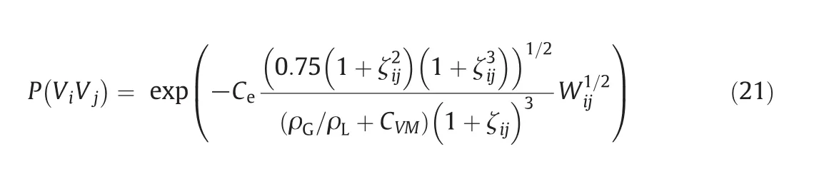
In this work,the coalescence resulted from turbulent eddies was considered.Turbulent eddies cause the bubbles to collide and coalesce with a certain probability.The mechanism of pressure on bubble coalescence is not yet clear.Up to now,models for bubble coalescence are mainly based on experimental phenomena by semi-theoretical semiempirical analysis.Wang[6]introduced a constant correction coefficient Cein the bubble coalescence model.But,we find that the correction coefficient Ceis not a constant under different gas velocities and pressures.In this work,according to the experimental data of Qin[14]from cold experiment,a density correction factor Cecan be obtained by simulation at the apparent gas velocity 0.199,0.233,0.275 m·s−1and the operating pressure at 0.5,1,1.5,2.0 MPa.Specific data are shown in Table 1.The linear regression equation between Ceand the gas density is as follow s:

Table 1Coalescence model correction coefficients and the simulated gas holdups

3.Geometric Model and Mesh Generation

The experiment of Qin[14]mainly examined the impact of pressure on the hydrodynamic behaviorsin variousoperating conditionsat 25°C.Air wasused asthe gasphase and water asliquid phase,the gas velocity was varied from 0.119 to 0.312 m·s−1and pressures from 0.5 to 2.0 MPa.

The geometry of the high-pressure bubble column is shown in Fig.1(a):height 6600 mm,diameter 300 mm,wall thickness5 mm.Tw o conductivity probes at the height of 2550 mm and 3050 mm are used to measure the bubble size in the radial direction and the velocity of rise of bubble groups.The electrodes of Electrical Resistance Tomography(ERT)are evenly mounted on the inner wall of the high-pressure bubble column at the height of 2600 mm and 3000 mm to measure the local air holdup and average gas holdup.

Compared with the 3D geometric model,the computational amount of the numerical simulation will be greatly reduced by the two-dimensional geometric model.Wang et al.[18]succeeded in simulating gas–liquid flow behaviors in a bubble column by an axisymmetric model.Therefore,two-dimensional axisymmetric geometric model are used in this work.As shown in Fig.1(b):6.6 m high and 0.15 m wide.In the model,no gas distribution plate is arranged on the column bottom and the gas is directly fed from the central bottom of the column(r/R≤0.8).The heights of 2550,2600,3000 and 3050 mm were set as the sampling sections.The experimental and simulation results are compared and analyzed in the following sections.

The mesh of 2D simulation structure is generated by the Mapped Face Meshing method.Modification of mesh at the wall:wall inflation,Maximum Layers:5,Grow th Rate:1.2.As shown in Fig.1(c),the obtained mesh is between the two sections from 2000 mm to 3200 mm above the bottom,and this section of 1200 mm length is enlarged to show the refine meshing at the wall.

In Fig.2,a grid independence verification was performed under the condition of 0.160 m·s−1and 0.5 MPa.The simulation results of radial gas holdup were compared and analyzed with four different grid fineness.This figure indicates that the simulation results with other three grids are basically consistent except for the first grid.Therefore,to ensure a high computing accuracy and an acceptable computing time,the grid with 5940 cells was adopted.

Fig.2.Effect of grid on the simulation results of gas holdup.

4.Results and Discussion

4.1.Gas holdup

4.1.1.Average gas holdup

Fig.3.Gas holdup at different apparent velocities and operating pressures(0.5,1.0,1.5,2.0 MPa).

The simulation results of the average gas holdup between the heights 2600 and 3000 mm at different apparent gas velocities and pressure were compared with the experimental data[14]in Fig.3.It is indicated that although the gas holdup made by the CFD-PBM coupled model without Cedirectly increases with the increasing apparent gas velocity,the error is greater than that by the modified CFD-PBM model with Cecorrection.It is shown that the modified CFD-PBM coupled model can accurately simulate the average gas holdup under other experimental conditions of Qin[14].

4.1.2.Radial gas holdup

In Fig.4,the simulated radial gas holdup profiles are compared with the experimental data under the operating conditions of 0.5,1.0,1.5,2.0 MPa and 0.160,0.215,0.253,0.317 m·s−1.The two diagrams at the same apparent velocity show the simulation results of the modified CFD-PBM coupled model and the CFD-PBM coupled model respectively compared with the experimental data.And the radial gas holdup showed a decreasing trend from the center to the column wall.It can be seen that the simulation results obtained by the CFD-PBM coupled model are generally smaller than the experimental data at elevated pressure.Luo et al.[32]proposed a model for the bubble interaction time by energy conservation analysis,ignoring the effects of operating pressures.If the Luo coalescence model is used directly to simulate high-pressure bubble column,as the simulation environment pressure is lower than the really pressure,the simulation result of gas holdup is smaller.It can be seen that when the density correction coefficient Ceis introduced into the Luo coalescence model,the error between the simulation results and the experimental data of Qin[14]is reduced.

4.2.Bubble diameter

4.2.1.Radial distribution of bubbles

Fig.5 describes the effect of operating pressure on bubble size radial distribution at the apparent gas velocity of 0.160,0.215,0.253,0.317 m·s−1.It can be seen from Fig.5 that although the bubble size decreases from the center to the edge of the column,the results obtained by the CFD-PBM coupled model are far larger than the experimental data at four different operating pressures(0.5–2.0 MPa)per gas velocity.On the other hand,the results obtained by the modified CFD-PBM coupled model are more consistent with experimental data.Therefore,the effect of operating pressure on the bubble diameter in the gas–liquid flow s can be well simulated by adjusting the density correction coefficient Cein the bubble coalescence model.

4.2.2.Bubble size distribution

Fig.6 shows the simulation results of the influence of pressure on the bubble sizedistribution at the apparent gas velocity of 0.160 m·s−1.The bubbles show a unimodal distribution.The number of medium bubbles(3–8 mm)increased at elevated pressure,while the number of smaller bubbles(＜3 mm)almost unchanged.It was consistent with the simulation results of Yang et al.[33].This is fully showed that the bubble size became smaller and more uniform at elevated pressure.

4.3.Velocity distribution

4.3.1.Air axial velocity

Fig.7 shows the effect of operating pressures on radial distribution of gas rising velocity.Simulation results at four gas velocities show a gradual decrease from the center to the column wall,and the gas velocity increases with the increase in the operating pressure and apparent gas velocity.The variation trend was consistent with the experiment reported by Wilkson et al.[34]

Fig.4.Gas holdup on radial distribution(u G=0.160,0.215,0.253,0.317 m·s−1).

4.3.2.Water axial velocity

Fig.8 shows the effect of pressure on the radial profiles of water axial velocity.It can be seen from Fig.8 that the axial liquid velocity gradually decreases from the center to the wall of the column.The liquid velocity is positive in the center of the column and negative near the side wall of the column.This indicates that the liquid phase appears to circulate in the column.The liquid circulation is in favor of gas–liquid fully contact.The difference in axial velocity is not significant at different operating pressures,indicating that the liquid velocity is not greatly affected by pressure.And the simulated results affected by pressure at other apparent gas velocities(0.215,0.253,0.317 m·s−1)are similar to result of 0.160 m·s−1.

Fig.5.Bubble diameter in the radial direction(u G=0.160,0.215,0.253,0.317 m·s−1).

5.Validation of the Modified CFD-PBM Coupled Model

The experiment of Wilkson and Dierendonck[34]mainly examined the influence of pressure on gas hold-up and bubble size in bubble column.The column had a diameter of 0.16 m,the height of column was 2.0 m.The liquid was deionized water(20°C),and gas was nitrogen.From the research of Reilly et al.[35]it is known that the influence of column diameter on gas-holdup can be neglected.So we choose the experimental data of gas-holdup versus superficial gas velocity for the water/nitrogen system[34]to validate the modified CFD-PBM coupled model.

Fig.9 shows the comparison between simulation results by the modified CFD-PBM coupled model and Wilkson's experimental data[34]under each pressure(0.5,1.0,1.5 MPa)at different apparent gas velocities.As can be seen,the simulation results of gasholdup are basically in agreement with the experimental data.So it shows that the modified CFD-PBM coupled model according to the experimental data of Qin[14]can be applied to the simulation under other experimental conditions.

Fig.6.Effect of operating pressure on bubble size distribution at 0.160 m·s−1.

6.Conclusions

The work focused on simulating the effects of operating pressure on hydrodynamic behavior.The CFD-PBM coupled model was employed to investigate the gas–liquid flow in a high-pressure bubble column.From the work,the following conclusions can be draw n:

Fig.8.Axial water velocity at different pressure simulated with C e(u G=0.160 m·s−1).

(1)From the comparison between experimental data and simulation results by two models(the CFD-PBM coupled model and the modified CFD-PBM coupled model),it can be seen that the latter model offers good agreement with experimental data.So the effects of operating pressure on the hydrodynamic parameters can be well predicted by the modified CFD-PBM coupled model.

(2)The effects of operating pressure on the bubble size distribution were predicted by the modified CFD-PBM coupled model in gas–liquid flow.The bubble size became smaller and more uniform at elevated pressure.

(3)Through the validation of the modified CFD-PBM coupled model with the water-nitrogen system of Wilkson and Dierendonck[34],it can be seen that the simulation results are in good agreement with the experimental results.So the modified model may be applied to other experimental systems.

Fig.7.Air axial velocity at different gas velocities and pressures.

Fig.9.Gas holdup under different apparent gas velocities.

Nomenclature

CDdrag coefficient

CD,∞ideal state drag coefficient

CLtransverse lift coefficient

CTDturbulent dispersion coefficient

CWLwall lubrication coefficient

dBdiameter of bubble,m

E0parameter E0

Fexinterphase forces

FDdrag force,N·m−3

FLtransverse lift,N

FTD,LFTD,Gturbulent dispersion force,N

fTD,limitingturbulent diffusion force model limiting function

FWLwall lubrication force,N

Gkturbulence energy generation

Gbk term of turbulent kinetic energy

g gravity acceleration,m·s−2

k,kLturbulent kinetic energy,m2·s−2

P operating pressure,Pa

Poatmospheric pressure under standard conditions,Pa

P(ViVj) bubble coalescence efficiency

Uivelocity,m·s−1,i=1:gas phase,i=2:liquid phase

uGgas velocity,m·s−1

uLliquid velocity,m·s−1

uijcharacteristic velocity of bubble collision

Ωbr(V,V′)bubble breakage rate

Ωag(ViVj)bubble coalescence rate,

εiphase holdup,i=1:gas phase,i=2:liquid phase

εGaverage gas phase holdup

εGgas phase holdup

εLliquid phase holdup

εG,1εG,2turbulent diffusion force limit function constant

ζijrelative diameter of bubble

ζminminimum relative diameter of bubble

μtturbulent viscosity,Pa·s

ρ0Gas density under standard conditions,kg·m−3

ρLliquid density,kg·m−3

ρGgas density,kg·m−3

σ surface tension,N·s−1

ω(ViVj) collision frequency between bubbles of size diand dj,m3·s−1