PENG Hanbang (彭汉帮) PAN Aijun (潘爱军) ZHENG Quan’an (郑全安) HU Jianyu (胡建宇)

1 State Key Laboratory of Marine Environmental Science, College of Ocean and Earth Sciences, Xiamen University, Xiamen 361102, China

2 Ocean Dynamics Laboratory, The Third Institute of Oceanography, State Oceanic Administration (SOA), Xiamen 361005, China

3 Department of Atmospheric and Oceanic Science, University of Maryland, College Park 20742, USA

Abstract This paper investigates the response of the thermocline depth (TD) in the South China Sea(SCS) to the El Niño-Southern Oscillation (ENSO) events using 51-year (from 1960 to 2010) monthly seawater temperature and surface wind stress data acquired from the Simple Ocean Data Assimilation(SODA), together with heat flux data from the National Centers for Environmental Prediction (NCEP),precipitation data from the National Oceanic and Atmospheric Administration (NOAA) and evaporation data from the Woods Hole Oceanographic Institution (WHOI). It is indicated that the response of the SCS TD to the El Niño or La Niña events is in opposite phase. On one hand, the spatial-averaged TDs in the SCS(deeper than 200 m) appear as negative and positive anomalies during the mature phase of the El Niño and La Niña events, respectively. On the other hand, from June of the El Niño year to the subsequent April, the spatial patterns of TD in the north and south of 12°N appear as negative and positive anomalies, respectively,but present positive and negative anomalies for the La Niña case. However, positive and negative TD anomalies occur almost in the entire SCS in May of the subsequent year of the El Niño and La Niña events,respectively. It is suggested that the response of the TD in the SCS to the ENSO events is mainly caused by the sea surface buoyancy flux and the wind stress curl.

Keyword: South China Sea (SCS); thermocline depth; El Niño-Southern Oscillation (ENSO); buoyancy flux; wind stress curl

1 INTRODUCTION

El Niño-Southern Oscillation (ENSO) over the tropical Paci fic Ocean is the strongest climate fluctuation on interannual and planetary scale with worldwide impacts. Generally, the warming phase is known as El Niño while the cooling phase as La Niña(Trenberth, 1997). The South China Sea (SCS),which is located in the East Asian monsoon region and close to the equatorial warm pool (Fig.1), is greatly in fluenced by the ENSO through teleconnections (i.e. “atmospheric bridge”) with in fluencing factors such as sea surface temperature(SST), sea surface winds, air temperature and humidity, as well as cloud cover and surface heat flux(Klein et al., 1999; Wang, 2002).

Fig.1 Bottom topography of the South China Sea

The in fluence of the ENSO events on the SCS (e.g.its hydrometeorology, temperature, heat flux and winds) has been investigated in previous studies. The response of the SST in the SCS to the ENSO events has been discussed by several investigators (Klein et al., 1999; Wang, 2002; 2006; Liu et al., 2014; Qiu et al., 2016). For example, Qiu et al. (2016) showed that the SST anomaly is positive and negative during the El Niño events in the southwestern and northeastern SCS, respectively, but conversely during the La Niña events. Kuo et al. (2004) attributed the response of the Vietnam coastal upwelling to the El Niño and La Niña events to the manifestation of the sea surface winds.Fang et al. (2006) indicated that the sea surface winds in the SCS are closely associated with the ENSO events at the interannual timescale. Yan et al. (2010)suggested that upper ocean heat content anomaly is usually positive while wind stress curl and latent heat flux are usually positive in the SCS during El Niño,and conversely during La Niña. However, response of the thermocline depth (TD) in the SCS to the ENSO events remains unclear. Changes in ocean heat content and strati fication are the key to understanding the dynamics of the SCS and the TD is an important indicative measure for them. According to previous studies, the TD in the SCS shows remarkable monthly and seasonal variability (Liu et al., 2001; Xiong,2012; Peng et al., 2017). Based on historical observation data, Hao et al. (2012) investigated the climatological seasonal variations of the thermocline in the China seas and northwestern Paci fic Ocean and regarded the sea surface buoyancy flux as the dominant driving mechanism for the TD variations.Using a coarse-resolution model of the Paci fic Ocean,Miller et al. (1997) showed that the modeled largescale thermocline anomaly is signi ficantly driven by large-scale Ekman pumping by interannual wind stress curl variations. Wang et al. (1999) suggested that the deepening and rising of the thermocline occur in phase with the local anticyclonic and cyclonic wind stress forcing in the tropical Paci fic, respectively.Using the Princeton Ocean Model (POM), Chu et al.(1999) argued that the seasonal variability of the TD in the SCS is affected by upwelling and downwelling.Based on the Simple Ocean Data Assimilation(SODA) data, Peng et al. (2017) examined the mechanisms causing monthly variation of the SCS TD, and the results reveal that the TD variations are in a good agreement with the sea surface buoyancy flux and wind stress curl. Based on the SCS Physical Oceanographic Dataset 2014 (SCSPOD14), Zeng et al. (2016) showed the monthly distribution of mixed layer depth (MLD), which is closely related to the TD, and found the MLD shows remarkable seasonal variations. Soon after, Zeng and Wang (2017)analyzed the seasonal variations of the barrier layer(BL) de fined by the MLD and ILD (isothermal layer depth, which is also related to the TD) in the SCS and the mechanism of BL variation, and the results reveal that the sea surface buoyancy flux and wind stress curl are the main physical mechanisms for the BL change. According to these results, we can conclude that the sea surface buoyancy flux and wind stress curl are the main mechanisms that can in fluence the TD in the SCS. As previously mentioned, the sea surface heat flux (the main component of buoyancy flux (Duan et al., 2012)) and the sea surface wind in the SCS can be in fluenced by the El Niño and La Niña events. Accordingly, a scienti fic question of interest is whether the El Niño or La Niña events can affect the TD in the SCS through those mechanisms. Therefore,in this study, we investigate the response of the TD in the SCS to the ENSO events and the possible physical processes.

The rest of the paper is organized as follows.Section 2 gives a brief description of the data and methods as well as the El Niño and La Niña records.Section 3 analyses the TD variability in the SCS associated with the ENSO events and the corresponding mechanisms. Section 4 shows the relationship between thermocline intensity in the SCS and Niño 3.4 index (hereafter N34). Section 5 gives the discussion and conclusions.

2 DATA AND METHOD

2.1 Data

The monthly seawater temperature, sea surface salinity and wind stress products used in this paper are from SODA (Carton et al., 2000a, b, 2005). The SODA model is based on observations including almost all available hydrographic pro file data, as well as ocean station data, mooring temperature and salinity time series, surface temperature and salinity observations of various types. The basic temperature and salinity observation sets consist of approximately 7×106pro files over the global ocean, of which two thirds have been obtained from the World Ocean Database 2009 (Giese and Ray, 2011), and the others include observations from the Tropical Atmosphere-Ocean/Triangle Trans-Ocean Buoy Network (TAO/TRITON) mooring thermistor array and Argo drifters.Output variables are averaged every five days, and then mapped onto a uniform global 0.5°×0.5°horizontal grid (a total of 720×330×40-level grid points), spanning the latitude range from 79.25°S to 89.25°N and the longitude range from 179.75°W to 179.75°E, using the horizontal grid spherical coordinate remapping and interpolation package(Carton and Giese, 2008). In this study, we use 50×50 pro files bounded by 0.25°–24.75°N and 100.25°–124.75°E and use the upper 25 vertical layers of the seawater temperature (from 5 to 1 625 m). The version of SODA used in our study is SODA v2.2.4 (Giese and Ray, 2011).

The sea surface buoyancy flux is calculated by the sea surface net heat flux and net fresh water flux (Gill,1982; Schmitt et al., 1989). The monthly net long wave radiation, net short wave radiation, sensible heat flux and latent heat flux data (1960–2010,1.875°×1.875°) used for the sea surface net heat flux calculation are downloaded from the National Centers for Environmental Prediction (NCEP) reanalysis(Kalnay et al., 1996) (ftp://ftp.cdc.noaa.gov/Datasets/ncep.reanalysis.derived/surface_gauss/). We use the monthly precipitation (1960–2010, 2.5°×2.5°) and evaporation data (1960–2010, 1°×1°) for the sea surface net fresh flux calculation. The monthly precipitation data are downloaded from the National Oceanic and Atmospheric Administration (NOAA)’s Precipitation Reconstruction (PREC) Dataset (Chen et al., 2002) (http://www.esrl.noaa.gov/psd/data/gridded/data.prec.html). The oceanic precipitation analysis (PREC/O) is produced by EOF (Empirical Orthogonal Function) reconstruction of historical gauge observations over islands and land areas. The monthly evaporation data are downloaded from Objectively Analyzed air-sea Fluxes (OAFlux)project (Yu et al., 2008) of Woods Hole Oceanographic Institution (ftp://ftp.whoi.edu/pub/science/oa flux/data_v3/monthly/evaporation/). The OAFlux project uses the objective analysis to obtain optimal estimates of flux-related surface meteorology and then computes the global fluxes by using the state-of-the-art bulk flux parameterizations.

2.2 Method

In this study, we adopt the gradient criterion method to determine the thermocline. The gradient criterion of thermocline is 0.05°C/m (General Administration of Quality Supervision, Inspection and Quarantine of the People’s Republic of China and Standardization Administration of the People’s Republic of China, 2008), i.e., the thermocline is de fined as the layer, from down to top, with the vertical gradient of temperature larger than 0.05°C/m for at least 5 consecutive meters. We de fine the depth of upper boundary of the thermocline as the TD.

The sea surface buoyancy flux, a comprehensive index of thermodynamics, re flects the coherent role of air-sea heat and haline exchanges (Gill, 1982; Schmitt et al., 1989). The buoyancy flux B (kg/(m·s3)) is calculated by

where Bqis the thermal buoyancy due to the net heat flux, Bpis the haline buoyancy due to the net fresh water flux, g is the gravitational acceleration, Q is the net heat flux (upward positive; W/m2), ρ is the reference water density and Cpis the speci fic heat of water, α is the thermal coefficient of expansion and β is the coefficient of haline contraction, S0, E, and P are surface salinity, evaporation and precipitation,respectively. If surface water loses heat (i.e., Q ＞0) or evaporation is greater than precipitation (i.e., E– P ＞0),the surface water will lose buoyancy that can enhance vertically convection and deepen the TD. On the other way, if surface water gets heat or precipitation is greater than evaporation, the surface water will get buoyancy that strengthens strati fication stability of the upper ocean and decreases the TD.

The monthly N34 is downloaded from the Climate Prediction Center of NOAA (http://www.cpc.noaa.gov/data/indices/ersst4.nino.mth.81-10.ascii). N34 is the averaged SST anomaly in the region bounded by 5°S to 5°N, from 170°W to 120°W and is one of the several ENSO indicators. Based on the criterion developed by the Climate Prediction Center of NOAA and de finition from Trenberth (1997), a 5-month running average of N34 exceeding +0.4°C or -0.4°C for at least 6 consecutive months is de fined as an El Niño or a La Niña event. According to this de finition,there are 9 El Niño events and 12 La Niña events from 1960 to 2010 (Table 1). In order to investigate the interannual variability of TD, the seasonal cycle must be removed. In this study, the monthly TD anomaly(TDA) is obtained by subtracting the monthly climatological mean value (from January of 1960 to December of 2010) from the TD.

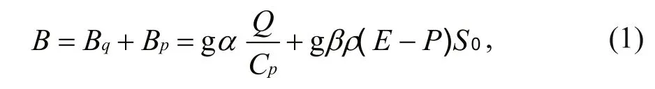
Table 1 The El Niño and La Niña events from 1960 to 2010

Fig.2 A comparison of the monthly TDA time series in the SCS (black line) with the El Niño events (shaded in orange) and La Niña events (shaded in blue) de fined by N34 from 1960 to 2010

3 THE TDA IN THE SCS ASSOCIATED WITH THE ENSO EVENTS

3.1 The spatial-averaged TDA in the SCS during the ENSO events

To obtain the spatial average of the SCS TDA, the TDA is averaged over the region with bathymetry deeper than 200 m in the SCS (Fig.1). Figure 2 shows the TDA and N34 time series in all calendar months from 1960 to 2010, the correlation coefficient between them is -0.46. One can see that the TDA varies in opposition with the El Niño and La Niña events, i.e.,the TDAs are negative during most time of the El Niño events, but positive during the La Niña events(except the 1984/1985 La Niña event).

Figure 3 shows comparisons between the TDA time series and N34 during the event year ([0]) and the event’s subsequent year ([1]) for 9 El Niño events and 12 La Niña events. As shown in Fig.3a, the SCS TDAs almost show the same evolution during 9 El Niño events, i.e., the TDAs are negative from October[0] to March [1] with the peak values in February [1],while are positive from April [1] to June [1] with the peak values in May [1]. On the contrary, during the La Niña events (except the 1984/1985 event) (Fig.3b) the TDAs are positive from September [0] to March [1]with the peak values in February [1], while are negative from May [1] to July [1] with the peak values in May [1]. Furthermore, from Fig.3c we can be more intuitive to see the opposite sign of TDA during El Niño and La Niña events.

It is noted that, as Fig.3c shows, the peak of the mean TDA in February [1] is lagged by two months with respect to the peak of the mean N34 in December[0] during the El Niño or La Niña event. This may result from the “atmosphere bridge” that connects the SCS with the SST anomaly in the central equatorial Paci fic, with some delay.

Fig.3 Comparisons between the spatial-averaged TDA in the SCS and N34 during 9 El Niño events (a) and 12 La Niña events (b), and the mean N34 and mean TDA averaged over all El Niño events and La Niña events (c) from 1960 to 2010 in the event year ([0]) and the event’s subsequent year ([1])

Fig.4 Zonal mean of composites of (a) TDA (units: m), (b)anomaly of B (units: 10 -5 kg/(m·s 3)), (c) anomaly of WSC (units: 10 -7 N/m 3) in the SCS from the El Niño year ([0]) to the subsequent year of the El Niño year([1])

3.2 The zonal average and the possible mechanisms of the SCS TDA

In Section 3.1 we have shown that the TDA in the SCS (spatially averaged TDA in the SCS) is in opposition with El Niño and La Niña SSTs (N34). In this section, we will further investigate the zonally averaged SCS TDA and the possible physical processes responsible for the TDA using composites of El Niño and La Niña events. Hereafter, we consider El Niño and La Niña composites computed from events over 1960 to 2010. According to the composite N34 (the thick red curves in Fig.3), we de fine the period from June [0] to September [0], from October[0] to February [1] and from March [1] to May [1] as the onset, mature and decay phases of the El Niño event, and the period from May [0] to August [0],from September [0] to February [1] and from March[1] to June [1] as the onset, mature and decay phases of the La Niña event.

As mentioned in the introduction, the main mechanisms to in fluence TD in the SCS are the buoyancy flux ( B) and wind stress curl (WSC) on the sea surface. Lombardo and Gregg (1989) and Lozovatsky et al. (2005) suggested that B and wind stress on the sea surface are the main dynamic factors to in fluence the structure of the upper ocean. The loss of buoyancy in the upper ocean, which triggers convection, would deepen the thermocline. On the contrary, if the upper ocean gains buoyancy, the seawater stability would be strengthened inhibiting thermocline from deepening due to the more difficult vertical convection. In this study, positive or negative B means the upper ocean loses or gains buoyancy. In addition, the WSC also in fluences the TD by Ekman pumping. Positive WSC, which triggers upwelling,can make the thermocline shallower. Conversely,negative WSC can deepen the thermocline through downwelling. In short, positive B tends to increase the TD while positive WSC tends to decrease the TD.

Figure 4 shows composites of zonally-averaged thermocline depth anomalies (TDAs), buoyancy flux( B) and wind stress curl (WSC) anomalies during the El Niño events in the SCS, as a function of latitude and time. Unlike the spatial average from Fig.3, the zonally-averaged TDA is not consistently negative during the El Niño events or positive during the La Niña events over the entire SCS. Instead, the evolutions of TDA in the northern and southern SCS (taking the 12°N as the boundary) are different. As shown in Fig.4a, the TDA is negative in the northern SCS but positive in the southern SCS from June [0] to April [1]during the El Niño event, especially from December[0] to March [1], when the TDA reaches -30 to -20 m north of 16°N. In May [1], the TDA is positive almost in the entire SCS (except in the region north of 18°N).

In order to explain the above phenomenon, we also show the composites of zonally-averaged anomaly of B (Fig.4b) and WSC (Fig.4c) during the El Niño event. The TDA tends to be positive when anomaly of B is positive or anomaly of WSC is negative, and to be negative when anomaly of B is negative or anomaly of WSC is positive. As Fig.4b and c show, at the onset of the El Niño event from June [0] to September [0],the anomaly of B is negative in the northern SCS and positive in the southern SCS, while the anomaly of WSC is conversely positive in the northern SCS and negative in the southern SCS. From October [0] to March [1], the mature phase of the El Niño event, the anomaly of B is negative in the northern SCS but positive in the southern SCS. In particular, the larger negative TDA north of 16°N from December [0] to March [1] may be due to the larger negative anomaly of B and positive anomaly of WSC. Later in May [1],the decay phase of the El Niño event, the positive anomaly of B and negative anomaly of WSC are the primary causes for the positive TDA nearly in the entire SCS (except in the region north of 18°N).

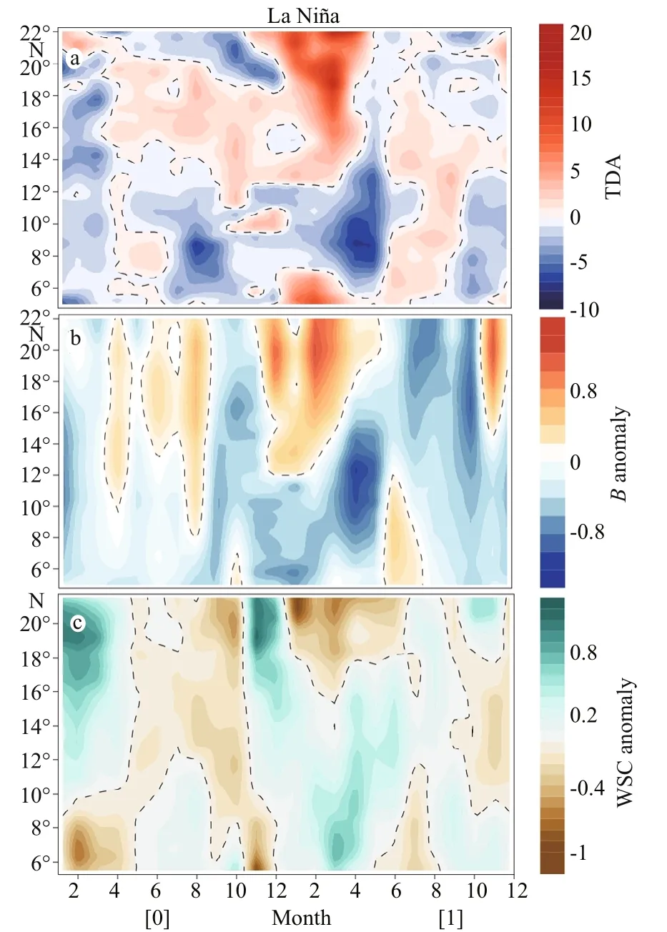
Fig.5 The same as Fig.4, but for the La Niña event

Figure 5 shows the composites of zonally-averaged TDA, the anomaly of B and WSC in the SCS during the La Niña events. One can see that the zonallyaveraged TDA, anomaly of B and WSC from June [0]to May [1] during the La Niña events are almost opposite of those during the El Niño events as shown in Fig.4, except in the region north of 18°N from June[0] to October [0] for the TDA, and the region north of 12°N from August [0] to November [0] and the region south of 12°N from February [1] to May [1]for the anomaly of B.

3.3 Spatial distribution of TDA and its mechanism in the SCS during the ENSO events

The TDA in most of the SCS, either spatially averaged or zonally averaged, appears almost in opposition with the El Niño and La Niña SSTs and has different values at different stages (the onset,mature and decay phases) of the El Niño or La Niña events. We select August [0], February [1] and May[1] as the representative month of the onset, mature and decay phases of the El Niño or La Niña event to investigate the spatial structures of TDA, together with the anomaly of B and WSC in the SCS.

Figure 6 shows longitude-latitude maps of composite TDA, anomaly of B and WSC at different stages (onset, mature and decay phases) of the El Niño events. In August [0] of the El Niño event, the TDA is negative in the northern SCS, but positive in the southern SCS (Fig.6a1). At the same time, the pattern of anomaly of B (Fig.6b1), which is negative in the northern SCS but positive in the southern SCS,is nearly the same with that of the TDA. Furthermore,the anomaly of WSC (Fig.6c1) is positive in most of the northern SCS, but appears negative in the southern SCS. In February [1] of the El Niño event, the TDA becomes more intense than that in August [0].Meanwhile, the positive TDA in the southern SCS expands northward (Fig.6a2). The anomaly of B, like the TDA, is more intense than that in August [0] and the positive values in the southern SCS expand northward (Fig.6b2), and the WSC anomaly in the southeastern and northwestern SCS is negative and positive (Fig.6c2), respectively. In May [1] of the El Niño event, the TDA is positive almost in the entire SCS except in the northeastern SCS (Fig.6a3).Correspondingly, the anomaly of B is positive almost in the entire SCS (Fig.6b3). Besides, the anomaly of WSC is negative almost in the SCS except the positive anomaly on the continental shelf break (Fig.6c3).

Figure 7 shows the spatial distributions of composite TDA, anomaly of B and WSC at different stages (onset, mature and decay phases) of the La Niña events. During the La Niña event, the TDA,anomaly of B and WSC nearly appear as opposite modes with those during the El Niño event, except in the region south of 12°N for the anomaly of B.

4 THE RELATIONSHIP BETWEEN THERMOCLINE INTENSITY (TI) IN THE SCS AND N34

As one of the indicative parameters of thermocline,the TD in the SCS presents pronounced variation during the ENSO events. Other indicative parameters of thermocline in the SCS, such as the thermocline thickness and intensity could also be in fluenced by the ENSO events. We analyze here the evolution of the thermocline intensity (TI) in the SCS and find that it shows a good correlation with N34.

Fig.6 Composites of TDA (units: m) (a1–a3), anomaly of B (units: 10 -5 kg/(m·s 3)) (b1–b3), anomaly of WSC (units: 10 -7 N/m 3)(c1–c3) in the SCS in August [0], February [1] and May [1] of the El Niño event

The TI is de fined as the average intensity over the thermocline, namely the ratio of the temperature difference and the depth difference between the upper and lower boundaries of the thermocline.

Figure 8 shows the lag correlation coefficient between the TI anomaly (TIA) and N34, and the time series of spatially-averaged TIA in the SCS and N34 during the same period. The TIA averaged over the SCS shows a lag correlation with N34 and the highest correlation coefficient is 0.63, when the TIA lags N34 for 5 months (Fig.8a). Figure 8b shows the time series of the spatially averaged TIA and N34 at the same period and the correlation coefficient is 0.41 (see Fig.8a). From the spatial distribution of the correlation coefficients between TIA and N34 in the SCS (Fig.9),one can see that the correlation coefficients increase gradually and the larger ones become wider from -5 to 5 months that TIA lags N34. It is noted that the correlation coefficient in the southeastern SCS (0.30–0.50) is larger than that in the northwestern SCS (0–0.20). The reason for such a feature deserves further study in the near future.

Fig.7 The same as Fig.6, but for the La Niña event

5 CONCLUSION AND DISCUSSION

In this study, the changes in thermocline depth(TD) in the South China Sea (SCS) associated with the El Niño-Southern Oscillation (ENSO) events during 1960 to 2010 and the mechanisms have been investigated. The main conclusions are as follows.

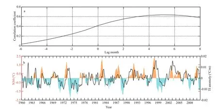
Fig.8 Lag correlation between spatially averaged TIA in the SCS and N34 (a), a positive lag means N34 is leading TIA; time series of spatially averaged TIA in the SCS and N34 (shading) during the same period (b)

Fig.9 Correlation between N34 and the SCS TIA at a lag of -5 months (a), 0 months (b) and 5 months (c)

(1) There are 9 El Niño events and 12 La Niña events that happened from 1960 to 2010 according to the criterion proposed by the Climate Prediction Center of NOAA based on N34. The TD anomalies in the SCS are in opposite with El Niño and La Niña SSTs for all those events (except the 1984/1985 La Niña event).

(2) By compositing the SCS TDA during 9 El Niño events, we find that the TDA averaged over the SCS is negative from the onset to mature phase of the El Niño event, but positive at the decay phase. The spatial patterns of the TDA are negative in the northern SCS and positive in the southern SCS during the onset phase, more intense during the mature phase, but become positive over the entire SCS in the decay phase.

(3) By compositing the SCS TDA during 12 La Niña events (except the 1984/1985 La Niña event),we find that the TDA averaged over the SCS is positive from the onset to mature phase of the La Niña event, but negative in the decay phase. The TDA, for the spatial patterns, is positive and negative during the onset phase in the northern and southern SCS,respectively, more intense during the mature phase,but becomes negative over the entire SCS in the decay phase.

(4) The main reason for the opposite sign of the TDA with respect to El Niño and La Niña SSTs is that the SST anomaly on the Tropical Paci fic Ocean,denoted by N34, can in fluence the buoyancy flux ( B)and the wind stress curl (WSC) on the sea surface of the SCS, which are the main mechanisms to affect the TD in the SCS, through the “atmospheric bridge”.

The TDA, anomaly of B and WSC show the reverse mode between the northern and southern SCS during the mature phase of El Niño and La Niña events. That may be due to the following aspects. (1) Qu et al.(2004) argued that the Luzon Strait transport can play a role in conveying the import of ENSO to the SCS.This may in fluence the haline exchanges or the heat content, which can in fluence B, and then the TD in northern SCS. (2) Due to the in fluenced wind stress over the SCS during ENSO and the different topographic effect around SCS, the anomaly of WSC may also present different over the northern and southern SCS and hence the TD.

Both B and WSC can in fluence TD in the SCS, but B is dominant (Hao et al., 2012; Peng et al., 2017).For the spatially average, TD matches B better than WSC during each individual ENSO event, except for the 1971/1972 La Niña event and the 2004/2005 and 1991/1992 El Niño events, of which both B and WSC are in a good agreement with TD. For the spatial distribution, the TDA is very similar to the composite mode during most of the ENSO events. The TDA north of SCS, however, is more intense and expands southward during the strong ENSO events (1997/1998 El Niño event and 1973/1974 La Niña event), anomaly of B and WSC are the same (not shown).