NONLINEAR STABILITY OF VISCOUS SHOCK WAVES FOR ONE-DIMENSIONAL NONISENTROPIC COMPRESSIBLE NAVIER–STOKES EQUATIONS WITH A CLASS OF LARGE INITIAL PERTURBATION∗
2018-07-23ShaojunTANG唐少君LanZHANG张澜
Shaojun TANG(唐少君)Lan ZHANG(张澜)
School of Mathematics and Statistics,Wuhan University,Wuhan 430072,China
E-mail:shaojun.Tang@whu.edu.cn;zhanglan@whu.edu.cn
Abstract We study the nonlinear stability of viscous shock waves for the Cauchy problem of one-dimensional nonisentropic compressible Navier–Stokes equations for a viscous and heat conducting ideal polytropic gas.The viscous shock waves are shown to be time asymptotically stable under large initial perturbation with no restriction on the range of the adiabatic exponent provided that the strengths of the viscous shock waves are assumed to be sufficiently small.The proofs are based on the nonlinear energy estimates and the crucial step is to obtain the positive lower and upper bounds of the density and the temperature which are uniformly in time and space.
Key words One-dimensional nonisentropic compressible Navier–Stokes equations;viscous shock waves;nonlinear stability;large initial perturbation
1 Introduction
The compressible Navier–Stokes system describing the one-dimensional motion of a viscous heat-conducting perfect polytropic gas in the Lagrange variables can be written in the following form
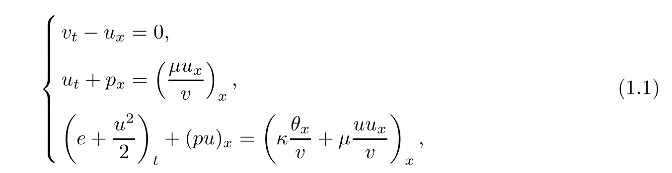
where t>0 is the time variable,x∈R is the spatial variable,and the primary dependent variables are the specific volume v, fluid velocity u,and absolute temperature θ.e is the specific internal energy.The viscosity coefficientµ and the heat conductivity coefficient κ are assumed to be positive constants.Here,we focus on the ideal polytropic gas,that is,the pressure p and the specific internal energy e are given by the constitutive relations

where s is the entropy,A is a positive constant,R>0 is the gas constant,and the specific heat cv=R/(γ−1)with 1<γ≤2 being the adiabatic exponent.
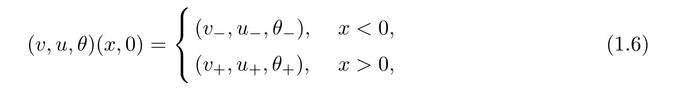
The system(1.1)is supplemented with the initial data

which are assumed to satisfy

where v±>0,u±and θ±>0 are given constants,and we assume infRv0>0,infRθ0>0,andas compatibility conditions.To describe the strengths of the shock waves for later use,we set

where δ∈ (0,1)is a constant.When the far field states are the same,that is,v+=v−,u+=u−,θ+= θ−,there has been considerable progress on the global existence of the solutions to system(1.1)since 1977;see[19,20,25–27]and the reference therein.In particular,Jiang[19,20] first obtained some interesting results on the large-time behavior of solutions,however the temperature is only shown to be locally bounded in space.More recently,Li and Liang[27]improved Jiang’s results by proving that the temperature is uniformly bounded.
The existence and large time behavior of solutions to system(1.1)with different end states become much more complicated.It is noted that,if the dissipation effects are neglected,that is,µ=k=0,system(1.1)is reduced to the compressible Euler equations as follows:
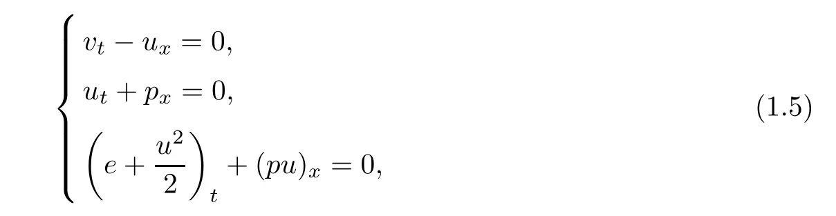
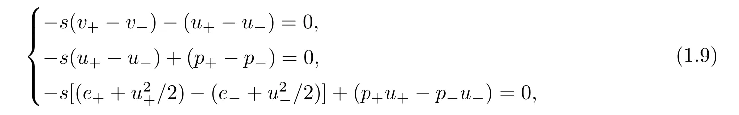
which is the most important hyperbolic system of conservation laws.It is well known that system(1.5)has rich wave phenomena.Indeed,it contains three basic wave patterns(see[38]),two nonlinear waves:shock and rarefaction wave,and a linearly degenerate wave:contact discontinuity.When we consider the Riemann initial data
the solutions consist of the above three wave patterns and their superpositions,called by Riemann solutions,and govern both the local and large time asymptotic behavior of general solutions of system(1.5).It is of great importance and interest to study the large-time behavior of the viscous version of these basic wave patterns and their superpositions to the nonisentropic compressible Navier-Stokes system(1.1).
For the nonlinear stability of some elementary wave patterns to the one-dimensional nonisentropic compressible Navier-Stokes systems,for the case with small initial perturbation,the results available up to now is quite complete except the cases when the elementary wave patterns are a linear superposition of one viscous shock pro file and one rarefaction wave or viscous contact discontinuity(for the nonlinear stability of viscous shock waves,see[23,33]for results with zero mass assumption and[28]for the case with general initial perturbation;for nonlinear stability of viscous contact discontinuities,see[14,30]with zero mass assumption and[17]for general initial perturbation;for the nonlinear stability of rarefaction waves,see[24,29];while for the nonlinear stability of composite wave patterns consisting of either rarefaction waves and viscous contact discontinuities or viscous shock waves from different families,see[11,13]).While for the corresponding results with large initial perturbation,some results are obtained for rarefaction waves(cf.[1,35–37]),viscous contact discontinuities(cf.[5,8,18]),and their superpositions(cf.[9,16]).But for viscous shock pro files,just Wang et al[41]used the argument developed by Kanel’in[22]to get the nonlinear stability of viscous shock pro files for the one-dimensional isentropic compressible Navier-Stokes equations.For the nonisentropic case,to the best of our knowledge,no results are available up to now.
To deduce the desired nonlinear stability result by the elementary anergy method as in[13,23],it is sufficient to deduce certain uniform energy type estimates on the solutions and the main difficulty to do so lies in how to control the possible growth caused by the nonlinear terms.For general γ>1,the arguments employed in[13,23]used the smallness of the initial perturbation and the strengths of viscous shock waves to overcome such a difficulty.One of the key points in such an argument is that,on the basis of the a priori assumption that the initial perturbation is sufficiently small,one can deduce a uniform lower and upper bounds on the specific volume v(t,x)and temperature θ(t,x).With such bounds in hand,one can thus deduce certain a priori H2(R)energy type estimates on solutions in terms of the initial perturbation provided that the strengths of the viscous shock waves are suitably small.The combination of the above analysis with the standard continuation argument yields the local stability of weak viscous shock waves for one-dimensional compressible Navier-Stokes equations.It is easy to see that in such a result,for all t∈R,Oscthe oscillation of specific volume v(t,x)and temperature θ(t,x),should be sufficiently small.For the global stability of viscous shock waves,the story is quite different.The main difficulty lies in how to deduce the uniform lower and upper bounds on the specific volume v and temperature θ under large initial perturbation.
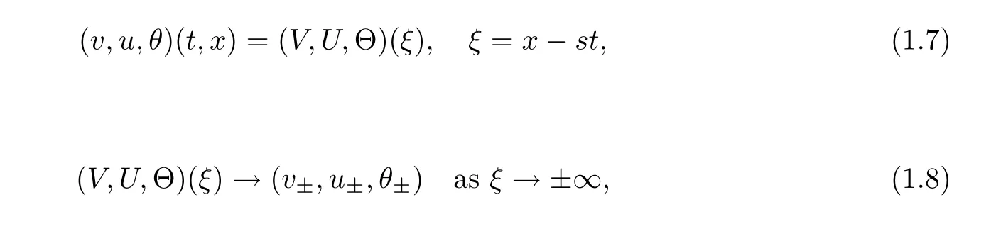
In this article,we establish the large-time behavior of solutions toward traveling wave solutions to(1.1)–(1.4)under large initial perturbation without any restriction on the adiabatic exponent γ.We expect that the solution converges to smooth traveling wave solutions with shock pro file
and the Lax’s shock condition that


To describe the strength of the shock wave for later use,we set

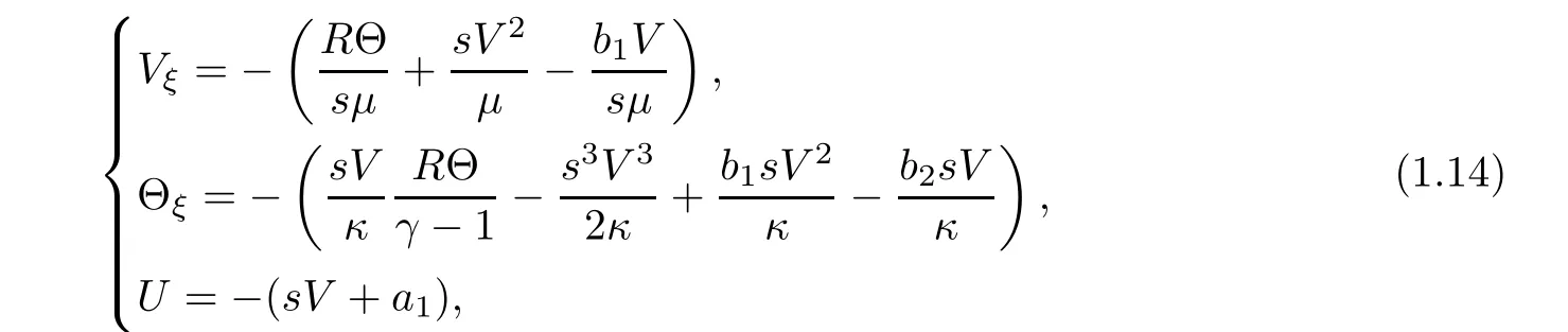
The functions(V,U,Θ)are determined by

In order to use the compressibility of the viscous shock pro files,we need to use the antiderivative technique.We reformulate the Cauchy problem to one for an integrated system in terms of the perturbation form(V,U,Θ)and put the perturbationby
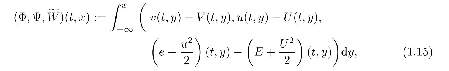
and we can assume that the initial data further satisfyFrom(1.15),we naturally look for the solution of(1.1)in the form

We have the following integrated system for
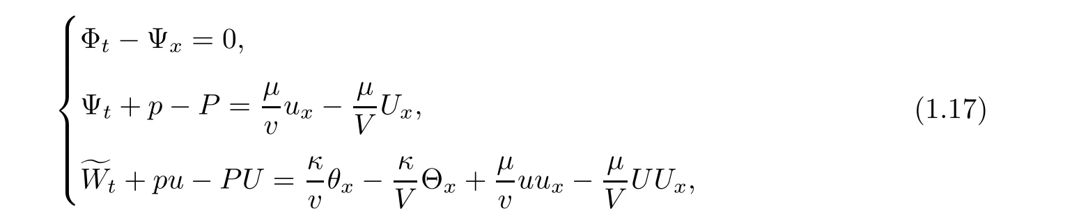
which replaces(1.16)by

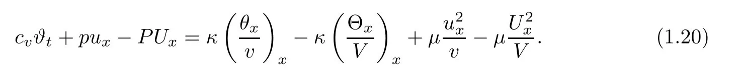
so we transfer system(1.17)into
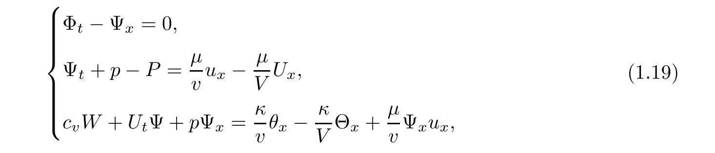
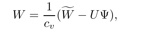
and we can rewrite(1.19)3as
Now,we turn to state our main result.First,we list some assumptions on the initial data(v0(x),u0(x),θ0(x)),the strength of the viscous shock δ:(H0)there exist δ-independent constants l1≥ 0,l2≥ 0,and C>0 such that

For simplicity,we assume that l1=l2=l in the following.(H1)v−,v+,θ−,and θ+are positive constants independent of δ.(H2)the initial data(v0,u0,θ0)are assumed to satisfy

Under the above assumptions,we have
Theorem 1.1Let v±,u±,θ±,and s be the given constants satisfying(1.9)and(1.10),let(V,U,Θ)(ξ)be a traveling wave solution which smoothly interpolates the asymptotic values(v±,u±,θ±)with speed s.Assume further that

If the δ-independent positive constants C0,α,and β are assumed to satisfy

then,there exist positive constants δ and ǫ,which are independent ofsuch that ifthen the initial value problem(1.1)and(1.3)has a unique global solution(v,u,θ)(t,x)with
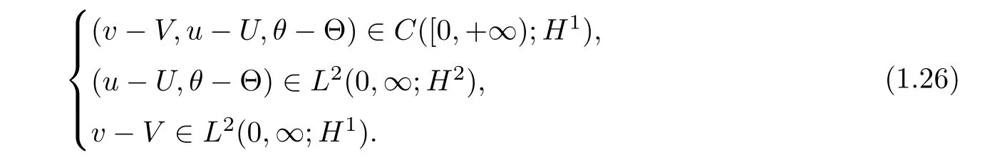
Moreover,the solution tends to the traveling wave solution in the maximum norm

Remark 1.2Some remarks concerning Theorem 1.1 are listed below:
• It is easy to see that the set of the parameters α >0,β >0,l≥ 0 which satisfy the assumption(1.25)is not empty.In fact,let l=0 andone can deduce that(1.25)is equivalent to,and the existence of such α and β is easy to verify.
• If the parameter α,β,l satisfy 3α − 3β − 6C0l<0,then for δ>0 sufficiently small,we can deduce from(2.110)that for each fixed t≥ 0,the oscillation of θ(t,x),can be large.
• For the simplicity of presentation,we assume that v−,v+,θ−,and θ+,the far fields of v0(x)and θ0(x),are independent of δ.For the case when the large time behavior of the global solution(1.1)is described by the superposition of viscous shock pro files of different families,similar result can also be obtained even when the far fields of v0(x)and θ0(x)depend on δ.
For the proof,we need some properties of traveling wave solutions.We first note that Rankine-Hugoniot condition(1.9)gives

for v+−V−>0,and

for v+−V−<0,wherewith
Lemma 1.3The traveling wave solution(V,U,Θ)(ξ)satisfies sand sΘξ<0 for any ξ∈ R.Moreover,there is a constant C independent of γ andsuch that for ξ∈ R,
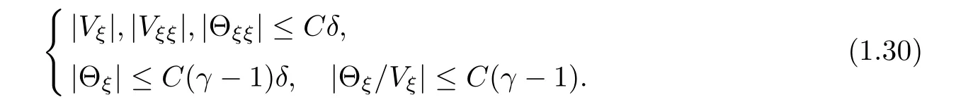
The estimate in(1.30)can be shown by direct calculations.We omit the proof.
2 A Priori Estimates
2.1 Reformation of the problem
This section is devoted to deriving a priori estimates on the solution(v,u,θ)to the Cauchy problem(1.1)–(1.3).We rewrite system(1.19)in form of(Φ,Ψ,W)as in the form

where(v,u,θ)is given by(1.18)and
and the initial condition(Φ0,Ψ0,W0)satisfies

The solution space X(0,T;m2,M2;m3,M3)is defined by

We denote here

For notational simplicity,we introduceif A≤CB holds uniformly for some positive constant C.All the positive constants c and C are independent of the strength of viscous shock waves δ.Besides,we will use the notation(v,θ)=(Φx+V,ϑ + Θ)so that

Without loss of generality,we may assume that mi≤1≤Mifor i=2,3.
2.2 Basic energy estimate
Our first result is concerned with the basic energy estimate,which is stated in the following lemma.
Lemma 2.1There exists a sufficiently small positive constant ǫ independent of δ such that if 0< δ≤ ǫ,then it holds that

with
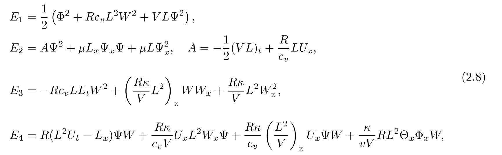
here and in the sequel,the notion(···)xrepresents the term in the conservative form so that it vanishes after integration.Because it has no effect on the energy estimates,we do not write them out in the details for simplicity.We estimate Ei,i=2,3,4,term by term.
We first note that


We further obtain

therefore,we get the following inequality for E2with the help of the Cauchy inequality,

For E3,because
then using the Cauchy inequality again,we have
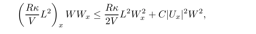
and we get

Next,for small δ,the Cauchy inequality gives

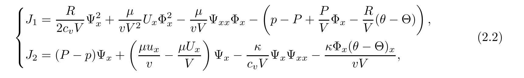
We now estimate the terms J1Ψ and J2W.From(2.2),we have the integrals of these terms on(0,t)×R as follows
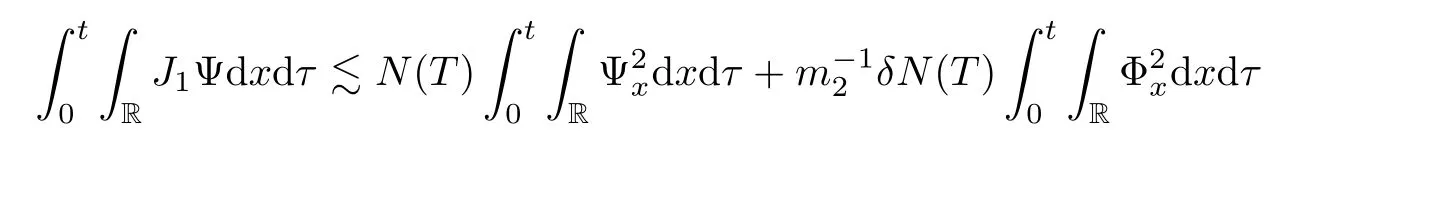
and

Integrating(2.8)on(0,t)×R,using(2.10),(2.12),and(2.13)–(2.16),we complete the proof of Lemma 2.1. ?
Lemma 2.2There exists a sufficiently small positive constant ǫ independent of δ such that if 0< δ≤ ǫ,then it holds that
where

ProofBy a straightforward calculation,we find

where
Integrate(2.19)over[0,T]×R to drive

From the Cauchy inequality,and the a priori assumption,we obtain the followings:


With above,we finish the proof of Lemma 2.2.
Notice that
A suitably linear combination of(2.6),(2.17),and(2.21)yields
Lemma 2.3There exists a sufficiently small positive constant ǫ independent of δ such that if 0< δ≤ ǫ,then it holds that

and by Cauchy’s inequality,we have

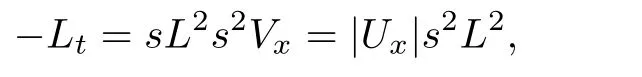
From(1.17),we have

where we have used the fact that Ux<0.
Integrating the above inequality with respect to t and x over[0,t]× R,and from Cauchy’s and Hölder’s inequality,we have
With(2.22)–(2.25),we have the following result.
Lemma 2.4There exists a δ-independent positive constant ǫ such that if

holds true,then we have,for each 0≤t≤T,
2.3 Pointwise estimates of specific volume
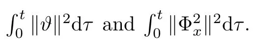
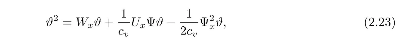
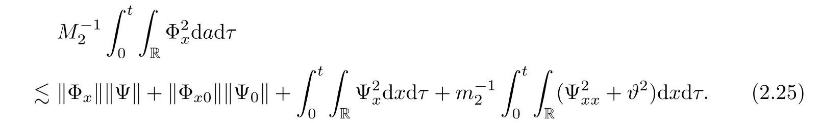
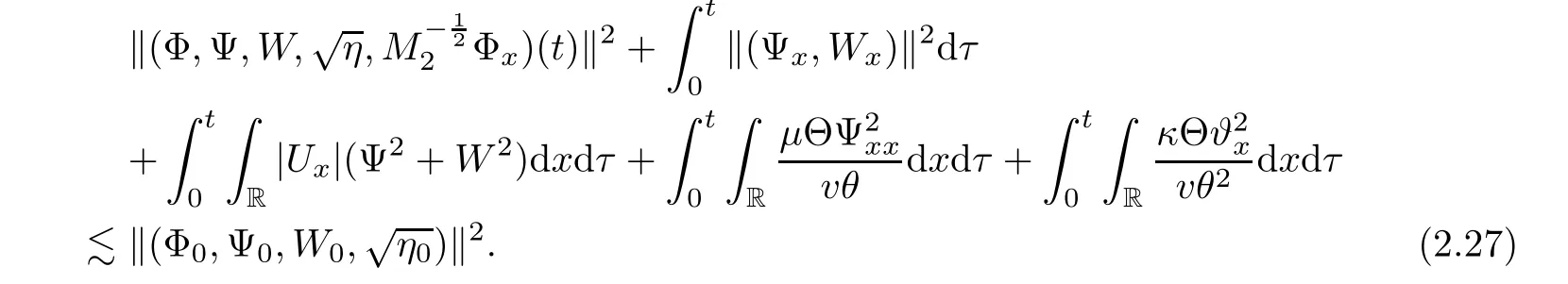
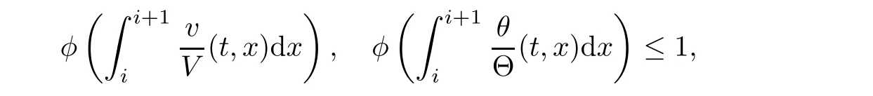
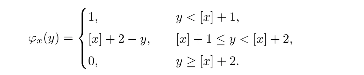
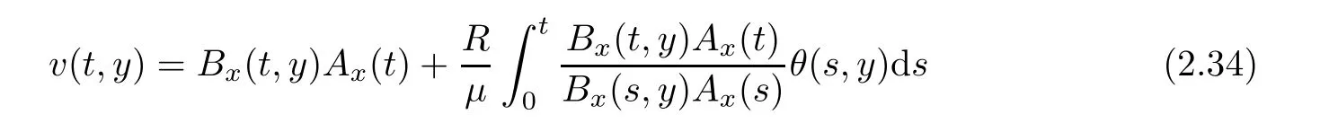
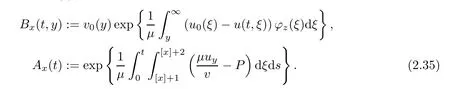
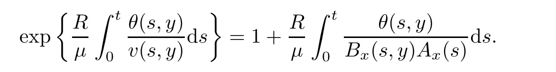
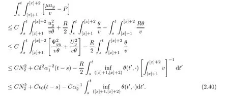
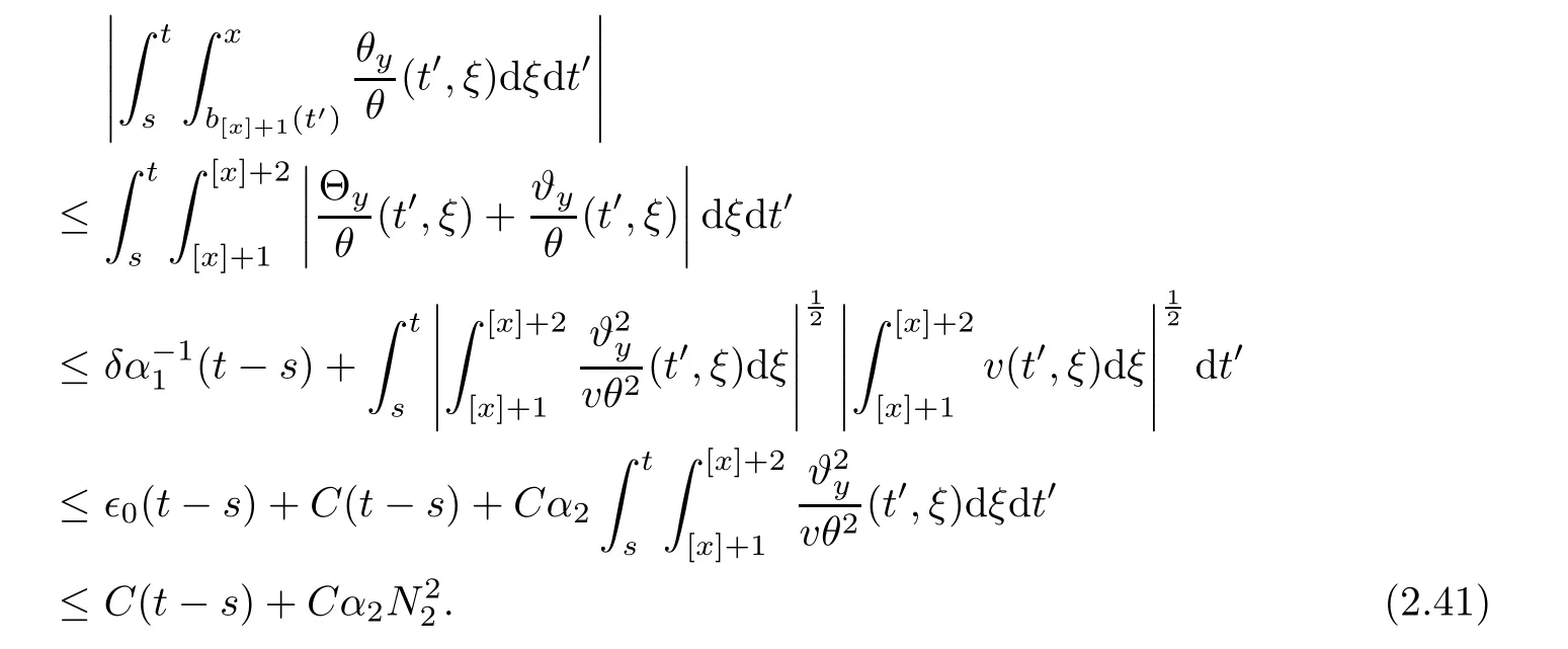
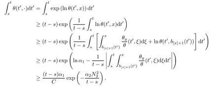
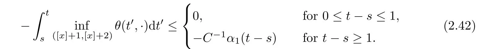
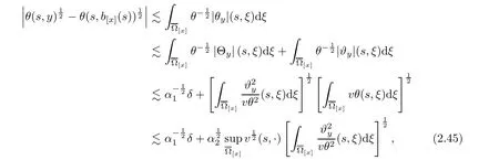
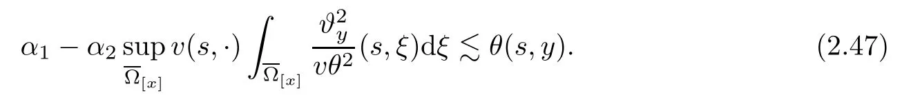
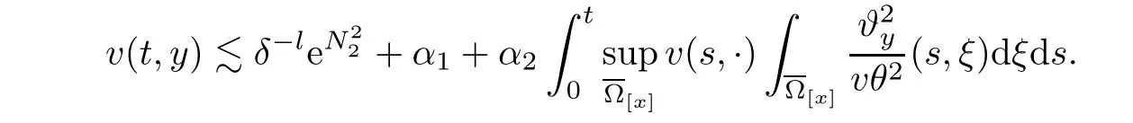
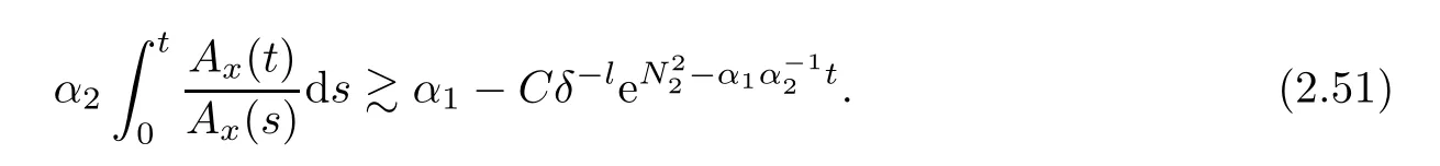
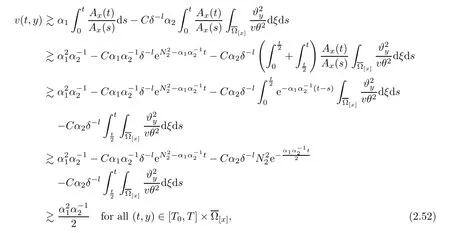
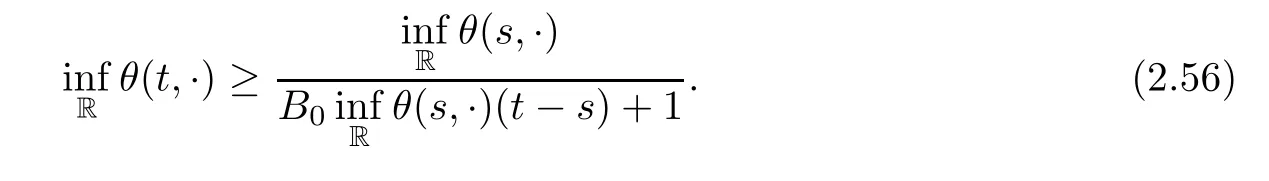
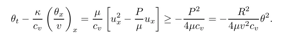
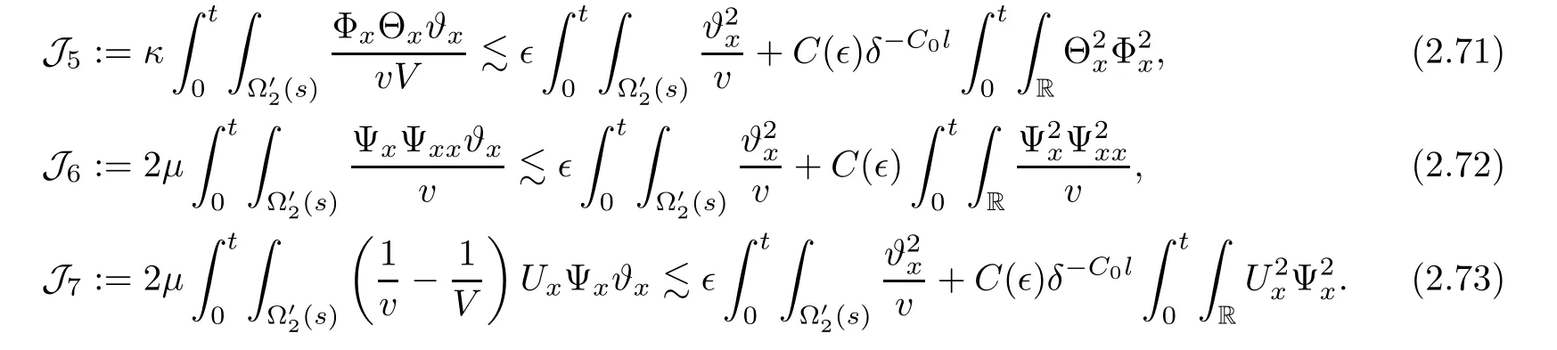
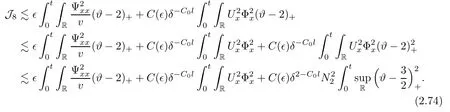
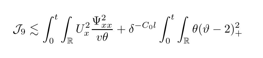
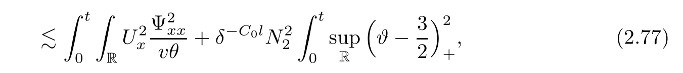
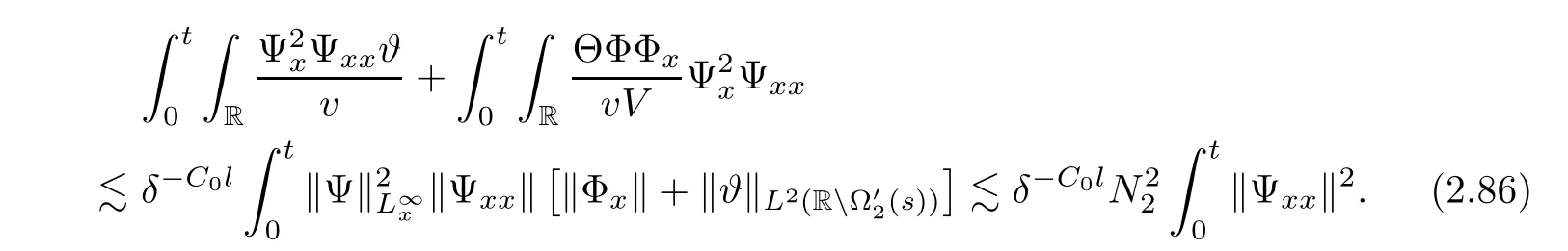
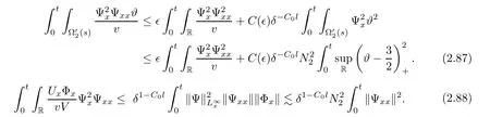
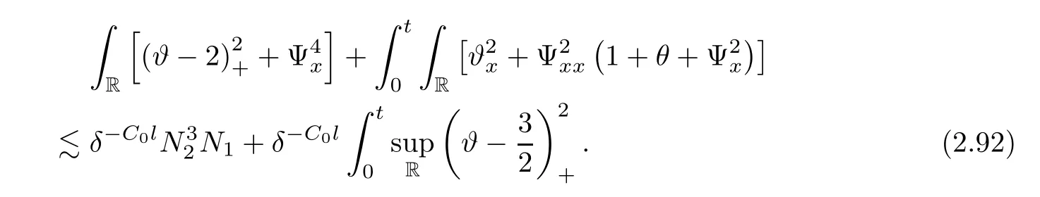
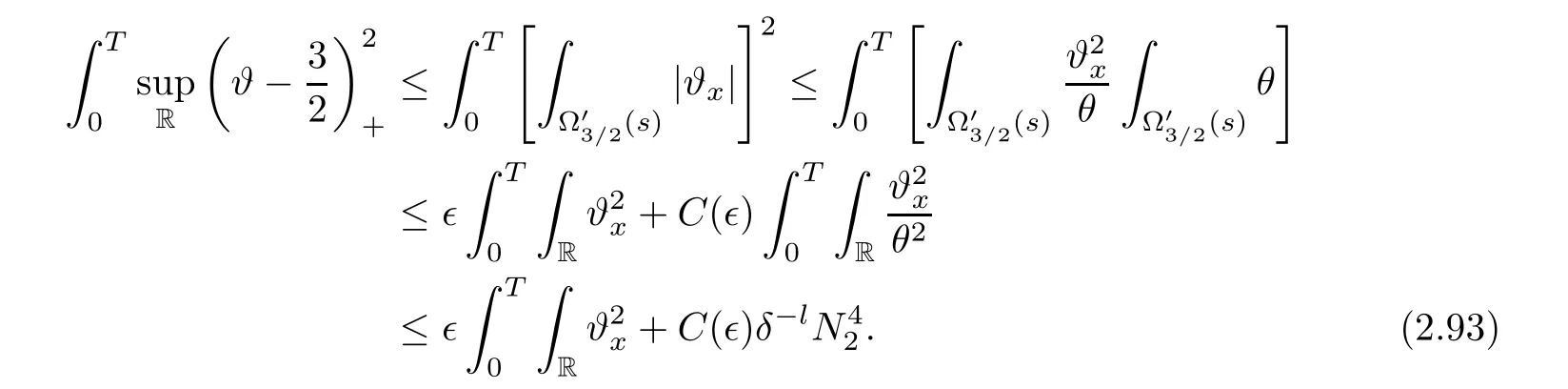
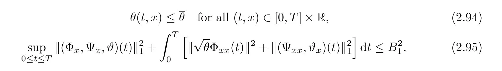
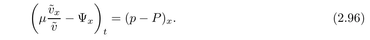
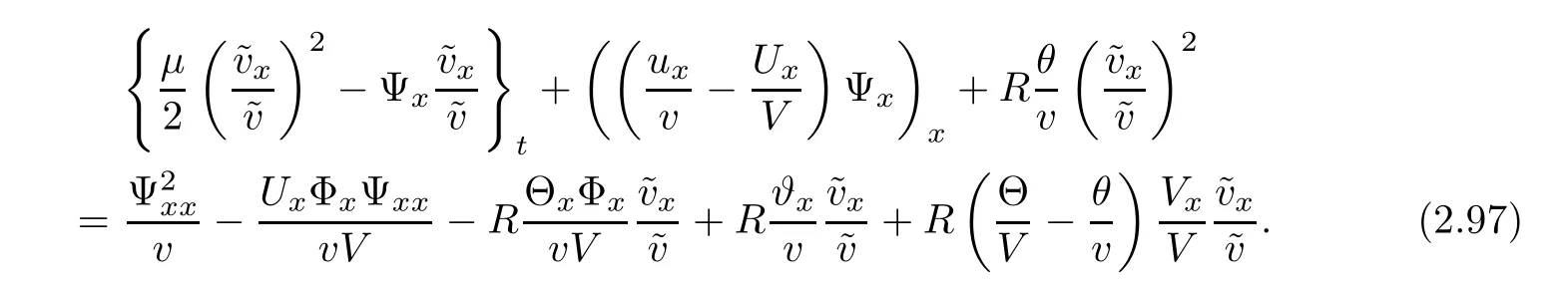
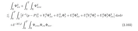
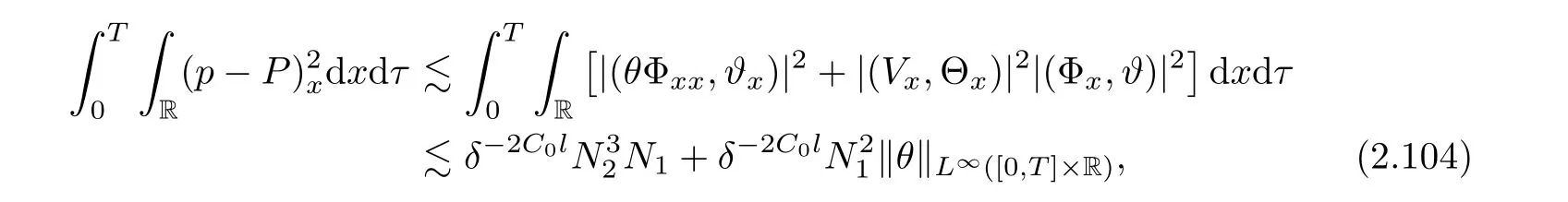
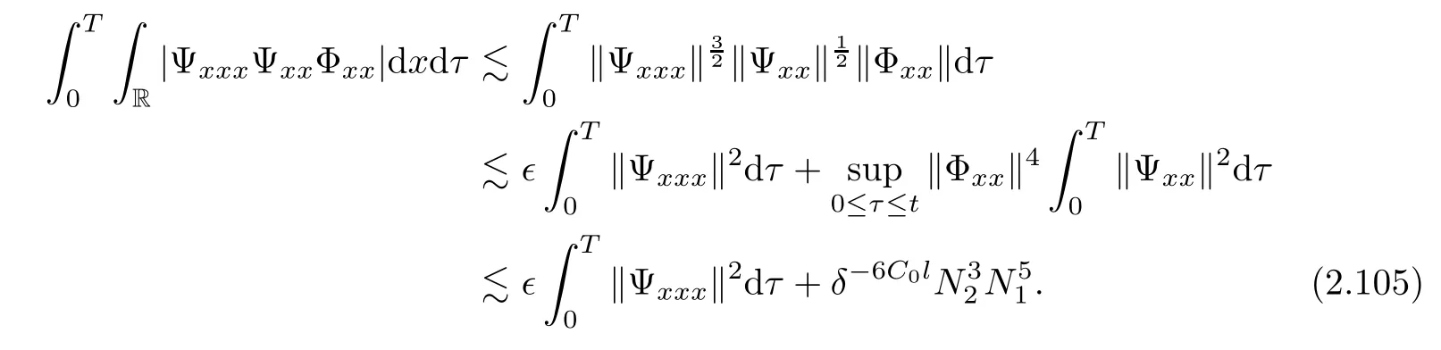
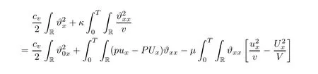
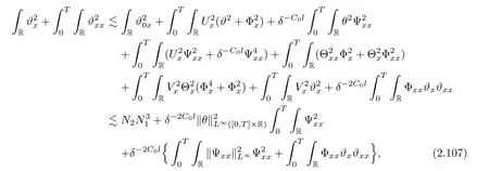
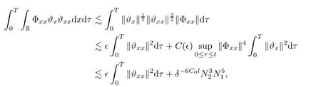
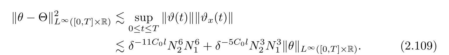
Notice the fact,for 0 then we first deduce from(1.21)that Hence,if(1.24)holds,then for 0<δ<1,α>l,we have Then with Lemma 2.4,we have the following corollary. Corollary 2.5For each time t∈[0,T],the following estimate holds: By Corollary 2.5,we see that where i=0,±1,±2,···for the Cauchy problem.Moreover,if we utilize(2.31)and apply Jensen’s inequality to the convex function φ,we obtain From above,we thus have proved Lemma 2.6Let α1,α2be two positive roots of the equation φ(x)=1.Then, and there are points ai(t),bi(t)∈[i,i+1]such that We deduce a local representation of v in the next lemma by modifying Jiang’s argument in[19,20]for fixed domains.To this end,we introduce the cutoff function ϕx∈ W1,∞(R)with parameter x∈R by For simplicity,we denote Ω[x]:=([x]− 1,[x]+1),then we have the following lemma. Lemma 2.7We have ProofWe multiply(1.1)2by ϕxto get In view of the identity ϕx(y)=1 and(1.1)1,integrating(2.36)over[0,t]× [y,∞),we obtain This implies that for each t∈[0,T], Multiplying(2.37)by Rθ(t,y)/µ and integrating the resulting identity over[0,t],we have We then plug this identity into(2.37)to obtain(2.34)and complete the proof of Lemma 2.7.? Now,to bound v(t,x)pointwise,we first show the exponential decay of Ax(t),then we use representation(2.34)to obtain the following local uniform bounds on v. Lemma 2.8If(2.26)holds for a sufficiently small ǫ0>0,then ProofThe proof is divided into three steps. Step 1In view of Cauchy’s inequality and(2.30),we have Let 0 ≤ s ≤ t≤ T.Apply Cauchy’s inequality and Jensen’s inequality for the convex function 1/x(x>0)and use(2.30)and(2.31)to deduce By Hölder’s and Cauchy’s inequalities,Lemma 2.6,and(2.30),we see that for x ∈ [[x]+1,[x]+2], Applying Jensen’s inequality to the convex function ex,we have,from(2.33)and(2.41), This implies Plugging(2.42)into(2.40)and taking ǫ0>0 small enough,we have,for each s ∈ [0,t], According to definition(2.35),we then obtain Step 2Plugging(2.39)and(2.43)into(2.34),we infer and We plug(2.46)into(2.44)to obtain Applying Gronwall’s inequality to(2.48),we can deduce from(2.30)that where C>0 is some constant independent of t,T,and y.Noting thatwe deduce from(2.49)thatis arbitrary,we conclude Step 3On the other hand,in view of(2.32),(2.39),and(2.43),we integrate(2.34)onwith respect to y to find Consequently,we have Inserting(2.47),(2.50),and(2.51)into(2.44),we have where we can choose T0=C lnδ−land C is independent of t.In particular,estimate(2.52)implies As in[26],we can derive a positive lower bound for v,that is, When t=T0=lnδ−l,we have Thus,this completes the proof. In the following lemma,we employ the maximum principle to get the lower bound for the temperature,which does depend on the time t. Lemma 2.9Assume that condition(2.26)holds.Then,there exist positive constant B0depending only onand k(Φx,Ψx,ϑ)k1such that it holds for all 0 ≤ s ≤ t≤ T that ProofIt follows from(1.1)3that θ satisfies Hence,we deduce from(2.38)that and Applying the weak maximum principle for the parabolic equation,we havefor 0≤s≤t≤T and x∈R.This completes the proof of Lemma 2.9.Here,? Next,we have the L2-norm in both time and space of ϑx. Lemma 2.10If(2.26)holds for a sufficiently small positive constant ǫ0,then ProofWe divide the proof into five steps. Step 1First,for each t≥0 and a>0,we denote Then,it follows from(2.30)and(2.38)that To estimate the last term of(2.59),we multiply(1.17)2by 2Ψx(ϑ − 2)+and integrate the resulting identity over(0,t)×R to find Combining(2.60)and(2.59),we have where each term Jpin the decomposition will be defined below.We now define and estimate all the terms in the decomposition.We first consider In light of(2.27),we have From Cauchy’s inequality and(2.38),we obtain and and Let us define Because we have Because J5,J6,and J7are easy to estimate,we write them together Let us now consider the term then we deduce from(2.65)that With the help of(2.65)and(2.69),the terms are estimated by and For the term we apply Cauchy’s inequality and(2.65)to deduce We finally consider then to estimate J12,we apply Lebesgue’s dominated convergence theorem to find where the approximate scheme φη(ϑ)is defined by And we have With the above inequalities,we get,from(2.38), Step 3It is obtained from(2.30)that Combining(2.82)and(2.83),and choosing ǫ sufficiently small,we have Step 4To estimate the last term of(2.84),we multiply(1.17)2byand then integrate the resulting identity over(0,t)×R to have From(2.58)and(2.65),we have We then apply Cauchy’s inequality to derive Plugging(2.86)–(2.88)into(2.85),and taking ǫ sufficiently small,we derive from(2.26)that We note from(2.30)that Combination of(2.90)and(2.89)yields We plug(2.91)into(2.84)and choose ǫ suitable small to find Step 5It remains to estimate the last term of(2.92).According to the fundamental theorem of calculus,we have,from(2.65), Plug(2.93)into(2.92)and choose ǫ>0 suitable small to obtain(2.57).This completes the proof of the lemma. ? We obtain the upper bound for the temperature uniformly in both time and space in the next lemma,by combining Lemma 2.10 and some desired uniform estimates on the spatial derivatives of(Φ,Ψ,ϑ). Lemma 2.11If(2.26)holds for a sufficiently small ǫ>0,then we have ProofFirst,we set.Then,we can rewrite(1.17)2as Integrating(2.97)with respect to t and x over[0,t]× R and employing Cauchy’s inequality,Gronwall’s inequality,and Lemma 2.4,we obtain Because we have and from(2.98),we deduce Next,multiply(1.17)2by−Ψxxxto derive Integrating this last identity over(0,T)× R,from(2.38)and Cauchy’s inequality,we obtain We only show how to estimate the first term and the last term in the following,as the rest is easier.To do so,by Cauchy’s inequality,we have and by Sobolev’s inequality and Young’s inequality,it holds that Finally,we get the estimate Next,multiplying(1.20)by−ϑxxand integrating the resulting identity over(0,T)×R,we have By a straightforward calculation,which combined with(2.38)implies as we have and we then obtain Finally,it follows from(2.57)and(2.108)that This implies(2.94)by virtue of Cauchy’s inequality;that is Combine(2.101),(2.106)and(2.108)to give which together with(2.57)yields(2.95).This completes the proof of Lemma 2.11. In this section,we will prove Theorem 1.1,which concerns the stability of the traveling wave solution.For this purpose,we first summarize the local existence of solutions to the problem(1.17)in the following proposition,which can be proved by the standard iteration method. Proposition 3.1(Local existence) Suppose that the conditions in Theorem 1.1 hold.If there exist positive constants M1,λiand Λi(i=1,2)such that,andhold for all x∈R,then(1.17)admits a unique solutionfor some constant T0=T0(λ1,λ2,M1)>0 depending only on λ1,λ2,and M1. Next,we will give the proof of Theorem 1.1 in six steps by employing the continuation argument. Step 1We choose positive constants Π,λi,and Λi(i=1,2,3)such that k(Φ0,Ψ0,W0)k2≤ Π and where λ1= λ2=Cδland Λ1= Λ2=C(1+ δ−l).Setwhere B1is exactly the same constant as in(2.95).Applying Proposition 3.1,we see that there exists a constant such that problem(1.17)has a unique solution Letting 0< δ≤ δ1,from Sobolev’s inequality,we have Consequently, Then,we can apply Lemmas 2.8,2.9,and 2.11 with T=t1to obtain the result that the local solution(Φ,Ψ,W)constructed above satisfies that for each t∈ [0,t1], and Step 2If we take(Φ,Ψ,W)(t1,·)as the initial data,we can apply Proposition 3.1 and extend the local solution(Φ,Ψ,W)to the time interval[0,t1+t2]with Moreover,we have for all(t,x)∈ [t1,t1+t2]×R,where From(2.27)and(2.57),we have Take 0< δ≤ min{δ1,δ2}with By employing Lemmas 2.8,2.9,and 2.11 with T=t1+t2,then the local solution(Φ,Ψ,W)satisfies(3.1)and(3.2)for each t∈[0,t1+t2]. Step 3We repeat the argument in Step 2,to extend our solution(Φ,Ψ,W)to the time intervalAssume that 0< δ≤min{δ1,δ2}.Continuing,after finitely many steps we construct the unique solution(Φ,Ψ,W)existing on[0,T1]and satisfying(3.1)and(3.2)for each t∈[0,T1]. Step 4Becauseand Sobolev’s inequality yields and so We note here that Now,we apply Proposition 3.1 again by takingas the initial data.Then,we see that the solution(Φ,Ψ,W)exists onwithand satisfies then we can deduce from Lemmas 2.8,2.9,and 2.11 withthat for each timethe local solution(Φ,Ψ,W)satisfies(3.2)and Step 5Next,if we takeas the initial data,we apply Proposition 3.1 and construct the solution(Φ,Ψ,W)existing on the time intervalwithand satisfying Then,we infer from Lemmas 2.8,2.9,and 2.11 withthat the local solution(Φ,Ψ,W)satisfies(3.3)and(3.2)for eachBy assuming 0< δ≤min{δ1,δ2,δ3,δ4},we can repeatedly apply the argument above to extend the local solution to the time intervalFurthermore,we deduce that(3.3)and(3.2)hold for eachIn view of,we have shown that problem(1.17)admits a unique solution(Φ,Ψ,W)on Step 6We take 0<δ≤min{δ1,δ2,δ3,δ4}.As in Steps 4 and 5,we can findsuch that problem(1.17)admits a unique solution(Φ,Ψ,W)onwhich satisfies(3.3)and(3.2)for each,we have extended the local solution(Φ,Ψ,W)to[0,2T1].Repeating the above procedure,we can then extend the solution(Φ,Ψ,W)step by step to a global one provided that δ≤ min{δ1,δ2,δ3,δ4}.Choosing ǫ1=min{δ1,δ2,δ3,δ4},we then derive that problem(1.17)has a unique solution(Φ,Ψ,W)satisfying(3.2)and for each t∈ [0,∞). Therefore,we can find constant B2depends only onand k(Φx0,Ψx0,ϑ0)k1such that from which the large-time behavior(1.27)follows in a standard argument.This completes the proof of Theorem 1.1. AcknowledgementsThe authors express much gratitude to Professor Huijiang Zhao for his support and advice.


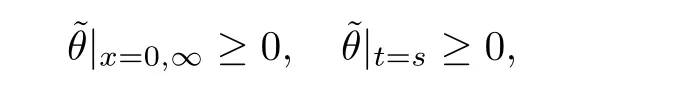
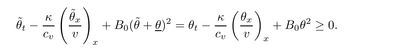
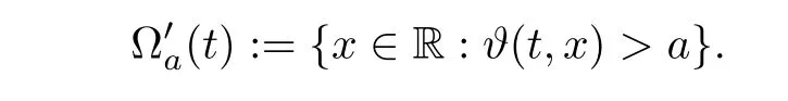
2.4 Pointwise estimates of temperature
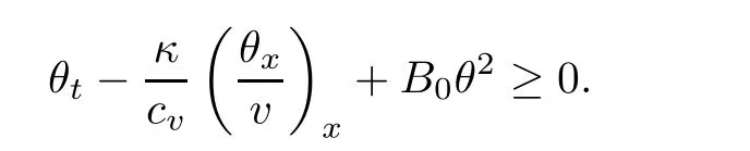


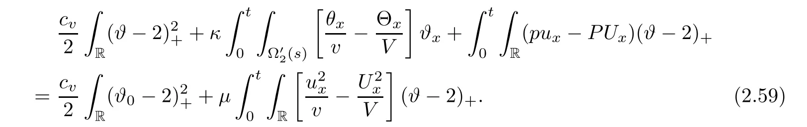
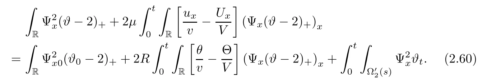
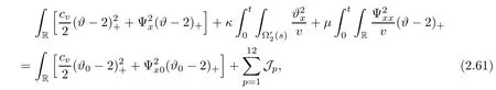
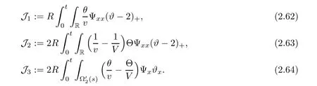


3 Proof of Theorem 1.1


杂志排行

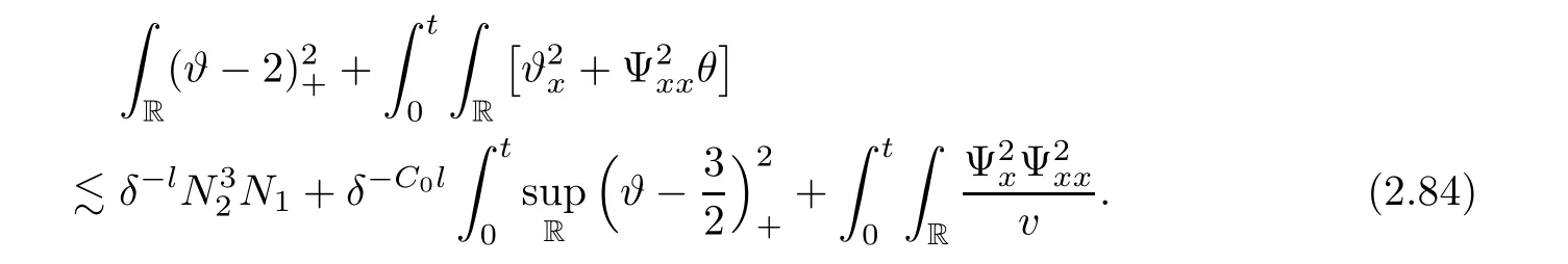
Acta Mathematica Scientia(English Series)的其它文章
- GLOBAL EXISTENCE OF CLASSICAL SOLUTIONS TO THE HYPERBOLIC GEOMETRY FLOW WITH TIME-DEPENDENT DISSIPATION∗
- NONNEGATIVITY OF SOLUTIONS OF NONLINEAR FRACTIONAL DIFFERENTIAL-ALGEBRAIC EQUATIONS∗
- GROWTH AND DISTORTION THEOREMS FOR ALMOST STARLIKE MAPPINGS OFCOMPLEX ORDER λ∗
- EXACT SOLUTIONS FOR THE CAUCHY PROBLEM TO THE 3D SPHERICALLY SYMMETRIC INCOMPRESSIBLE NAVIER-STOKES EQUATIONS∗
- PRODUCTS OF RESOLVENTS AND MULTIVALUED HYBRID MAPPINGS IN CAT(0)SPACES∗
- CONVERGENCE FROM AN ELECTROMAGNETIC FLUID SYSTEM TO THE FULL COMPRESSIBLE MHD EQUATIONS∗