EXACT SOLUTIONS FOR THE CAUCHY PROBLEM TO THE 3D SPHERICALLY SYMMETRIC INCOMPRESSIBLE NAVIER-STOKES EQUATIONS∗
2018-07-23JianlinZHANG张建材
Jianlin ZHANG(张建材)
Department of Applied Mathematics,College of Science,Zhongyuan University of Technology,Zhengzhou 450007,China
E-mail:mathzhangjianlin@hotmail.com
Yuming QIN(秦玉明)
Department of Applied Mathematics,Donghua University,Shanghai 201620,China
E-mail:yuming qin@hotmail.com
Abstract In this article,we establish exact solutions to the Cauchy problem for the 3D spherically symmetric incompressible Navier-Stokes equations and further study the existence and asymptotic behavior of solution.
Key words Navier-Stokes equations;asymptotic behavior;Riccati equation
1 Introduction
In this article,we consider the Cauchy problem for 3D spherically symmetric incompressible Navier-Stokes equations with no boundary and no external force in R3×(0,+∞)

where U=U(x,t)∈R3denotes the velocity field,P=P(x,t)∈R is the pressure of the fluid,and the viscosityµis a positive constant.Our aim here is to investigate the asymptotic behavior for a special class of solutions to problem(1.1).We assume that the corresponding solutions only depend on the radial variable r and the time variable t∈[0,+∞),that is,we study the solutions given by

where the radial variable r=|x|and u(r,t),p(r,t)both are scalar functions.Hence,the relevance of such solutions for the theory of the Navier-Stokes equations may be limited.Nevertheless,the behavior of these solutions provides an interesting insight into various scenarios of singularity formation.
After a direct calculation by(1.2),problem(1.1)is reduced to
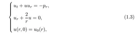
Equations(1.1)are a fundamental model in fluid mechanics and describe the motion of incompressible viscous flows.The mathematical study of problem(1.1)has a long history,which we shall describe briefly in this paragraph.We shall first recall results concerning the main global well posedness results,and some blow-up criteria.Then,we shall concentrate on the case when the special algebraic structure of the system is used.
There are numerous works on the theoretical studies,but,so far the global regularity problem of smooth solutions remains an outstanding open problem,that is,we do not know whether the smooth solutions will always exist or they break down at a finite time.
The weak solution to problem(1.1)was constructed by early works of Leray[42,43].Leray[43]proved that any finite energy initial data(meaning square-integrable data)generates a(possibly non unique)global in time weak solution which satisfies an energy estimate.Leray[42]proved the uniqueness of the solution in two space dimensions.Those results use the structure of the nonlinear terms,in order to obtain the energy inequality.He also proved the uniqueness of weak solutions in three space dimensions,under the additional condition that one of the weak solutions has more regularity properties(say belongs to L2(R+;L∞):this would now be qualified as a “weak-strong uniqueness result”).The question of the global well posedness of the Navier-Stokes equations was then raised,and has been open ever since.As far as we know,many works has also been published on various weak solutions;see[8,9,25,26,30,39,40,62]and the references therein.
The strong solution known with uniqueness is only local,or it exists only for sufficiently small initial data.Fujita and Kato[22]proved a unique,local in time solution in the homogeneous Sobolev spacein d space dimensions,and that solution is proved to be global if the initial data is small inWeissler[66]improved this result to the Lebesgue space Ld.Cannone,Meyer,and Planchon[19]also generalized this result to Besov spaces of negative index of regularity.They proved that if the initial data are small in the Besov(for p<+∞),then there is a unique,global in time solution.More recently,Koch and Tataru[35]obtained a unique global in time solution for data small enough in a more general space,consisting of vector fields whose components are derivatives of BMO functions.The existence of global generalized solutions with uniqueness for arbitrary initial data remains open.But,up to now,there are also many works on problem(1.1)with large initial data satisfying some special conditions.Especially,for large data,strong global solutions are known to exist only under the assumption of certain spatial symmetries,such as axial,rotational,and helical symmetry.Ladyzhenskaya[36]proved the global existence of rotationally symmetric large strong solutions in domains Ω⊂R3which are obtained by rotation about the x3-axis of a planar domain D lying in the half plane x2=0,x1>0 at a positive distance from the x3-axis,assuming the angular components of the force f and the initial data U0do not depend on the angle of rotation r about the x3-axis.Ukhovskii and Iudovich[64]proved the global existence of large strong axially symmetric solutions in the whole space.Axial symmetry is meant that the solution is rotationally symmetric and its component in the φ direction is zero.Feng andŠverák[21]considered the initial vorticity ω0concentrated on a circle,or more generally,a linear combination of such data for circles with common axis of symmetry,and proved the existence of global smooth solutions.Gallay andŠverák[23]considered the three-dimensional axisymmetric Navier-Stokes equations without swirl,using scale invariant function spaces,and showed the existence of a unique global solution,which converges to zero in L1norm as t→+∞ if the axisymmetric vorticity ωθis integrable with respect to the two-dimensional measure drdz,where(r,θ,z)denote the cylindrical coordinates in R3.Global existence for arbitrary large data on axisymmetric flows without swirl,see also[1,31,41,52]and the references therein.Mahalov,Titi,and Leibovich[47]established the existence of unique global strong solutions for large helically symmetric data.There,Ω is an in finite periodic pipe in the x3-direction with Dirichlet boundary conditions on the sides.Helical symmetry means that the solution U=U(r,φ,x3)in cylindrical coordinates actually only depends on r and nφ+αx3,where n ∈ Z{0}and α >0 are given parameters.Lei,Lin,and Zhou[37]derived a new energy identity for 3D incompressible Navier-Stokes equations by a special structure of helicity and constructed a family of finite energy smooth solutions whose critical norms can be arbitrarily large.Plecháč andŠverák[51]studied a dissipative nonlinear equation modelling certain features of the Navier-Stokes equations by penalization schemes method and proved that the evolution of radially symmetric compactly supported initial data does not lead to singularities in dimensions n≤4 and for dimensions n>4,it has strong numerical evidence supporting existence of blow-up solutions.Thus,it would be an interesting problem to study the global solvability of these “symmetric”solutions in the case of“large” initial data.
Naturally,it would also be an attracting problem to discuss the asymptotic behavior of these “symmetric” solutions.The connection between symmetry and space-time decay was first noticed in[4].Brandolese[4]showed that the localization condition L1(Rn,(1+|x|)dx)is instantaneusly lost if the data has non-orthogonal components with respect to the L2inner product.And he also obtained global strong solutions of problem(1.1)with an over-critical decay under the conditions of some supplementary symmetries of small initial data.Subsequentely,this problem was also studied in[5,49].Brandolese[6]showed that the solutions to the nonstationary Navier-Stokes equations in Rn(n=2,3),which are left invariant under the action of discrete subgroups of the orthogonal group O(n),decay much faster as|x|→ +∞ or t→ +∞than in generic case,and obtained,for each subgroup,the precise decay rates in spacetime of the velocity field.Gallay and Wayne[24]proved the existence of flows with a fixed,but arbitrarily large,time decay rate.Using the vorticity formulation of the Navier-Stokes equations,they showed that the class of solutions which decay faster than a given rate as t→+∞lies on an invariant manifold of finite codimension,in a suitable functional space.He and Miyakawa[29]studied the 3D exterior nonstationary problem and proved the L1-summability for smooth solutions which correspond to initial data satisfying certain symmetry and moment conditions.Furthermore,they showed that such solutions decay in time more rapidly than observed in general,and also obtained a lower bound estimate for the rates of decay in time.For the asymptotic behavior of the Navier-Stokes equations,Schonbek[58,59] first showed that ifthen the solutions U(x,t)to problem(1.1)decay at a rate ofRecently,Qin and Zhang[56]established exact solutions of the Cauchy problem for the 3D cylindrically symmetric incompressible Navier-Stokes equations and obtained the global existence and asymptotic behavior of solutions.We also refer the readers to[2,18,20,24,27,28,48,49,60,61,67]and references therein.
In addition,Chemin and Gallagher[13]provided new examples of arbitrarily large initial data giving rise to global solutions in the whole space and contrary to the previous examples,the initial data have no particular oscillatory properties,but vary slowly in one direction.In some sense,it is“well prepared”(its norm is large but does not depend on the slow parameter).Chemin,Gallagher,and Paicu[15]generalized the setting of[13]to an “ill prepared”situation(the norm blows up as the small parameter goes to zero).Analogous results to the classical Navier-Stokes system in the framework of small data are proved in[10–12,17,32,50].Recently,Tao[63]considered the averaged Navier-Stokes equation and proved the existence of finite time blowup solution.More results on the Cauchy problem for the Navier-Stokes equations,see[3,14,16,22,33,34,44,45,65,68]and the references therein.
Let us recall some related results on the Navier-Stokes system.For the compressible Navier-Stokes equations,Lions[46]not only established the existence of global weak solutions of initial boundary value problem of isentropic Navier-Stokes equations by approximation and compactness methods,but also constructed the global existence to the Cauchy problem by regularization and time discretization.Qin[53]established the global existence and large-time behavior of strong solutions to the one-dimensional polytropic gas and heat-conducting gas in Sobolev spaces.Especially,he also proved the similar results on a polytropic ideal gas in bounded annular domains and a polytropic viscous gas with cylinder symmetry in Rn.Qin and Huang[54]dealt with the global existence of spherically symmetric solutions for nonlinear compressible non-autonomous Navier-Stokes equations.Subsequently,Qin,Liu,and Wang[55]established exponential stability of spherically symmetric solutions to nonlinear non-autonomous compressible Navier-Stokes equations.For more similar results on some fluid models,such as MHD models,p-th power Newtonian fluid,micropolar fluid model,and radiative and reactive gas,see also[53–55,57,69]and the references therein.
Our purpose here is to investigate the existence and asymptotic behavior of exact solutions to problem(1.3).
We are now in a position to state our main theorems.
Theorem 1.1Let C(t)=u(1,t).If there exists a continuous function f(t)satisfying the Riccati equation
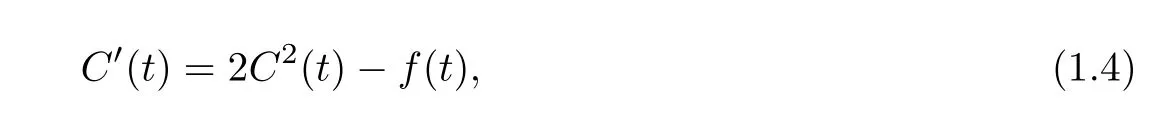
then problem(1.3)has a unique solution(u,p)such that for all(r,t)∈(0,+∞)×(0,+∞),it can be expressed as

and

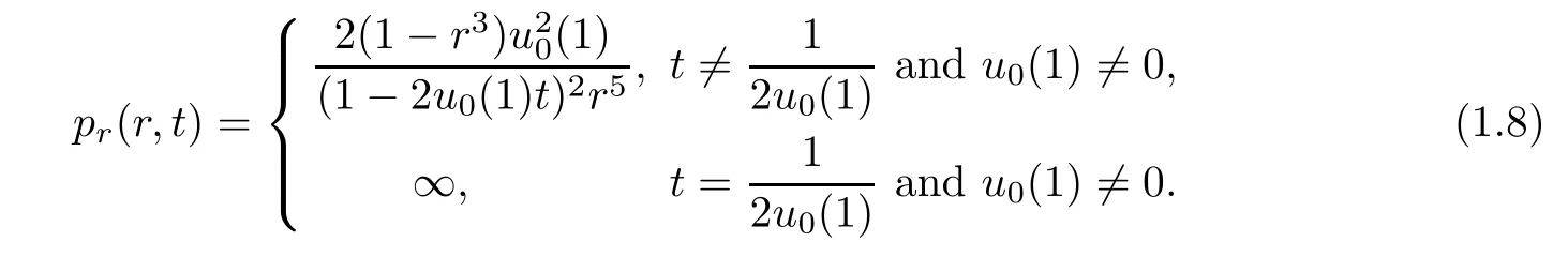
(i)If C(t)satisfies(1.4)with f(t)≡0,then problem(1.3)has a unique solution(u,p)which can be expressed as,for r>0,t>0,

and
(ii)If C(t)satisfies(1.4)with f(t)≡2C2(t),then we have

(iii) If C(t)satisfies(1.4)withsatisfyingthen,for all(r,t)∈(0,+∞)×(0,+∞),
(a)If f(t)is a positive function on[0,+∞),then

and
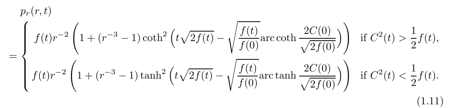
(b)If f(t)is a negative function on[0,+∞),then,
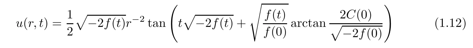
and

Theorem 1.2Under the assumptions of Theorem 1.1,a solution u(r,t)to problem(1.3)has following asymptotic behavior:


(ii) If C(t)satisfies the equation C′(t)=2C2(t),then solution u(r,t)has the time asymptotic behavior,that is,for any fixed r>0,

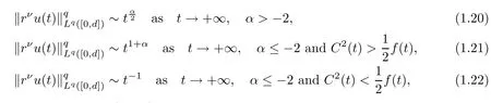
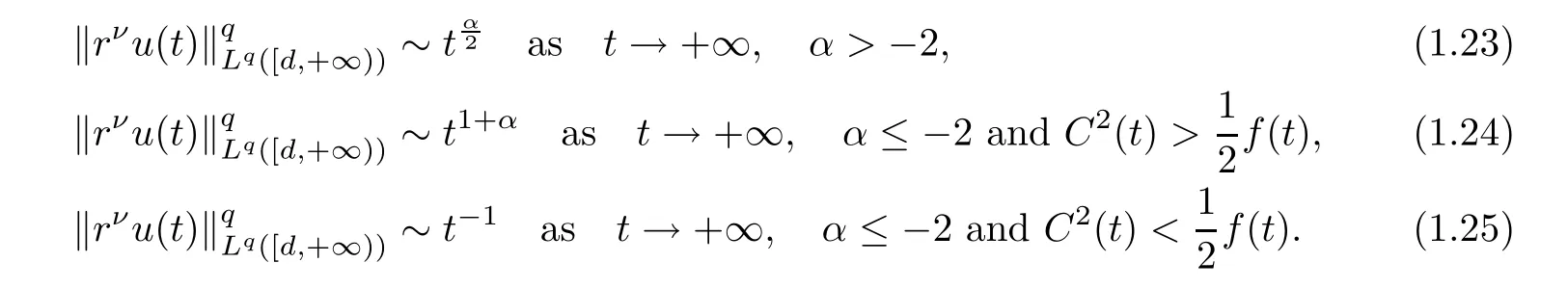
Theorem 1.3Let 1≤q<+∞.Under the assumptions of Theorem 1.1,a solution u(r,t)to problem(1.3)has the following decay rate on time:
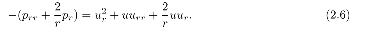
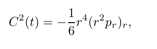
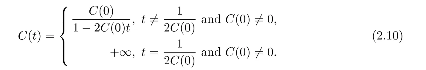
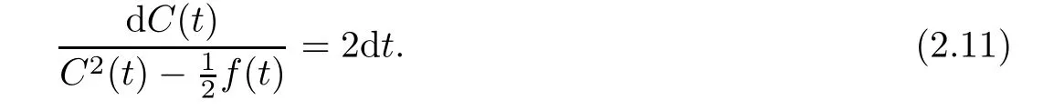
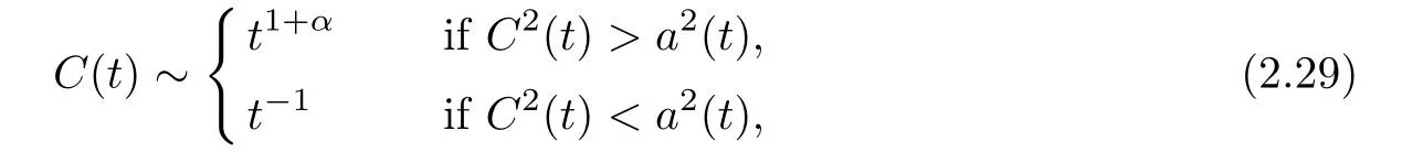
(i) If C(t)satisfies the equation C′(t)=2C2(t),then solution u(r,t)satisfies,for any 0 (ii)If C(t)satisfies(1.4)and there exists a constant α such that then solution u(r,t)has the decay rate on time as follows: (a)for any 0 (b)for any 0 (iii)If C(t)satisfies(1.4)and there exists a constant α such that then solution u(r,t)has the decay rate on time as follows: (a)for any 0 (b)for any 0 Remark 1.4It is worth pointing out that in this article we adopt a new and simple method to study the asymptotic behavior;that is,using the exact solutions which can be obtained in Theorem 1.1 and elementary analysis technique,we establish the asymptotic behavior in Theorems 1.2-1.3.Our results are not the special case in the previous work in[4,5,29,58–61]. From(1.5),we know that the properties of solutions u(r,t)depends on those of function C(t).While C(t)satisfies the ordinary differential equation(1.4)which is a Riccati equation,So,we can obtain our results from this Riccati equation.The first difficulty we encounter here is to derive the ordinary differential equation(1.4)from problem(1.3).To overcome it,we use the divergence-free condition to obtain(2.7)–(2.8)and then deduce the Riccati equation.The second difficulty is to solve the Riccati equation(1.4)because function f(t)is unknown.To overcome it,we give some special properties of unknown function f(t).The third difficulty is to establish the asymptotic behavior and time decay rate of solutions.To cope with it,we use the properties of hyperbolic tangent,hyperbolic cotangent,and tangent functions. In this section,we shall establish the existence of exact solutions to problem(1.3)by some lengthy calculations and discuss the decay estimates on time of solutions. In this subsection,we shall complete the proof of Theorem 1.1. ProofTo begin with,we derive the expression of the velocity u(r,t)from(1.3).It follows from(1.3)2that Let C(t)=u(1,t).Then,we solve the ordinary differential equation(2.1)in r and obtain Inserting(2.1)into(1.3)1yields Inserting(2.2)into(2.3),we can obtain that is, On the other hand,it follows from(1.1)that which,together with(1.2),leads to Inserting(2.2)into(2.6)implies that is, Let f(t)=pr(1,t).Then,integrating(2.7)with respect to r over[1,r],we obtain which,along with(2.4),yields the following equation Obviously,this is the special Riccati equation on C(t).Only if we can obtain a special solution to(2.9),we also obtain the solution to problem(1.3). Next,we shall solve equation(2.9). (i)Obviously,if f(t)≡0,then,it follows from(2.9)that Thus,noting C(0)=u0(1),(2.2),and(2.8),we obtain(1.7)–(1.8). (ii)If f(t)≡ 2C2(t),then C(t)=C(0)=u0(1).Furthermore,u(r,t)=u0(1)r−2and (iii)If f(t)6≡0 and f(t)6≡2C2(t),then we can rewrite equation(2.9)as Integrating(2.11)over(0,t)leads to Thus,we only need to calculate the right-hand side of(2.12)and then obtain the expression of C(t). Case If(t)>0. which,together with(2.13)and the definitions of hyperbolic functions,implies Inserting(2.15)into(2.2)and(2.8)yields(1.10)and(1.11). Case IIf(t)<0. which,together with(2.13),leads to Therefore,combining with(2.2),(2.8)and(2.16)yields(1.12)and(1.13). ? In this subsection,we shall deal with the asymptotic behavior of u(r,t)and give the proof of Theorem 1.2. (ii)Now,we cope with the time-asymptotic behavior of u(r,t),which depends only on the time-asymptotic behavior of C(t).It follows from(2.10)that Thus,for any fixed r>0,we obtain(1.16).? Now,we turn to prove Theorem 1.3. ProofLet 1≤q<+∞.Now,we shall estimate the time decay rates of u(r,t).First,we know that for any 0 and for any 0 It follows from(1.5)that we have,for any 0 and By virtue of(2.19)–(2.22),we know that the time decay rates of u(r,t)depends on the properties of C(t). (i)Obviously,(2.10)gives which,together with(2.19)–(2.22),leads to(1.17)–(1.18). (ii)By the definition of hyperbolic cotangent function,we know that Similarly,by the definition of hyperbolic tangent function,we also know that Thus,from(2.15),we have the followings: (1)When f(t)∼ tα(α > −2),as t→ +∞,it is obtained from(2.24)and(2.26)that,as t→+∞, which,together with(2.19)–(2.22),implies(1.20)and(1.23). which,together with(2.19)–(2.22),implies(1.21)–(1.22)and(1.24)–(1.25). By the definition of tangent function,we know that the tangent function is a periodic function and has the properties Thus,we deduce from(2.17)that which,along with(2.19)–(2.22),leads to(1.28)and(1.30).We thus complete the proof. ?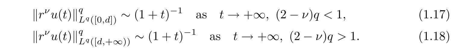


2 Proofs of Theorems
2.1 Proof of Theorem 1.1


2.2 Proof of Theorem 1.2

2.3 Proof of Theorem 1.3


猜你喜欢
杂志排行

Acta Mathematica Scientia(English Series)的其它文章
- GLOBAL EXISTENCE OF CLASSICAL SOLUTIONS TO THE HYPERBOLIC GEOMETRY FLOW WITH TIME-DEPENDENT DISSIPATION∗
- NONNEGATIVITY OF SOLUTIONS OF NONLINEAR FRACTIONAL DIFFERENTIAL-ALGEBRAIC EQUATIONS∗
- GROWTH AND DISTORTION THEOREMS FOR ALMOST STARLIKE MAPPINGS OFCOMPLEX ORDER λ∗
- PRODUCTS OF RESOLVENTS AND MULTIVALUED HYBRID MAPPINGS IN CAT(0)SPACES∗
- CONVERGENCE FROM AN ELECTROMAGNETIC FLUID SYSTEM TO THE FULL COMPRESSIBLE MHD EQUATIONS∗
- ON ENTIRE SOLUTIONS OF SOME TYPE OF NONLINEAR DIFFERENCE EQUATIONS∗