Kazunori Shinohara

1 Introduction

1.1 Leaf function

Trigonometric functions are generally used to mathematically describe a regular wave in terms of amplitude and period. The trigonometric functionssin(θ)andcos(θ)can be defined by using a unit circle. The coordinates (cos(θ), sin(θ)) represent the intersection point between the unit circle and the straight line obtained by rotating the positive part of thex-axis counterclockwise around the origin through an angleθ. Therefore, by using trigonometric functions, solutions are obtained on the basis of the structure of the unit circle. This often makes it impossible to derive exact solutions that satisfy nonlinear equations. Therefore, approximate expressions obtained using trigonometric functions are generally applied to nonlinear equations.

The solution of some ordinary differential equations through numerical analysis may have the characteristics of waves. However, exact solutions representing these waves almost always cannot be derived using trigonometric functions.

To derive an exact solution of various ordinary differential equations, it is necessary to define a new base function instead of trigonometric functions. This study considers very simple ordinary differential equations: the second derivative of a function and the power exponent of a function [Shinohara (2015)].

In this study, variablenis considered as the basis, which represents natural numbers (n=1,2, 3,…). Variablenin front of functionr(l)2n-1in Eq. (1.1) represents a coefficient for normalizing the unit amplitude of the wave. Variablelrepresents the phase. It is different from angleθexcept forn=1. As described later,lgeometrically represents the length of a curve (forn=1,lis equal toθ.) Through numerical analysis, we can obtain a solutionr(l)that satisfies ordinary differential equations. We find that the ordinary differential equations (Eqs. (1.1)-(1.3)) produce a regular wave (solutionr(l)) with a constant amplitude and period at all times. This wave is generated when the exponent ofr(l)is a positive odd number2n-1but not when the exponent ofr(l)is an even number2n. Forn=1in Eq. (1.1), a function that satisfies the ordinary differential equation represents the trigonometric functionsin(l). Forn=2in Eq. (1.1), the lemniscate functionsl(l)is satisfied, while forn ≥ 3, this function does not exist. As the basisnincreases, a regular wave converges to the following function.

Eq. (1.4) is therefore a discontinuous function. On the other hand, solutionr(l)forn=1,n=2, n=5, andn=10is shown in the graph. Asnincreases, the curve converges to the wave obtained using Eq. (1.4), and the period of the wave reaches 4.

Figure 1: Curves obtained by the ordinary differential Eqs. (1.1)-(1.3)(basis: n=1, n=2, n=5, and n=10)

Although the curve shows concavity and convexity in Fig. 1, the curves obtained using solutionr(l)are continuous. Such wave features obviously differ from those obtained using trigonometric functions. No conventional function satisfies the ordinary differential equations given by Eqs. (1.1)-(1.3). Therefore, the unknown function is defined as a leaf function as follows:

At this time, the relations amongx, y, andrare defined as follows:

The representation “sleaf” is combination of “sin” and “leaf.” The subscriptnrepresents the basis. As shown in Figs. 2-5, the numerical data (Tabs. 1 and 2) obtained using the functionsleafn(l)are plotted on a graph with variablex(Eq. (1.8)) along the horizontal axis and variabley(Eq. (1.9)) along the vertical axis. The curves obtained using leaf functions have a leaf-like shape, which is why the representation “sleaf” is used.

Figure 2: Geometrical relation among variables l, θ, and r for n=1

Figure 3: Geometrical relation among variables l, θ, and r for n=2

Figure 4: Geometrical relation among variables l, θ, and r for n=5

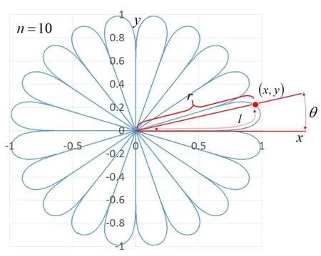
Figure 5: Geometrical relation among variables l, θ, and r for n =10

Table 2: Numerical data with respect to variable l (unit of parameter θ is °)

Variablesxandyobtained using Eqs. (1.8) and (1.9) always pass through the origin.Variablerrepresents the distance between the origin and the point (x, y). Variableθis the angle between thex-axis and the straight line connecting the point (x, y) and the origin.Variablelrepresents the length of the curve. Asnincreases, the number of leaves increases.

Leaf functionsleafn(l)is supposed to be an extension of the trigonometric functionsin(θ).It is assumed that a similar system can be extended using trigonometric functioncos(θ).

We define the ordinary differential equations that satisfy another leaf function as follows:

The function satisfying the ordinary differential equations is represented ascleafn(l). Forn=1,cleaf1(l)represents trigonometric functioncos(l). Forn=2,cleaf2(l)represents lemniscate functioncl(l). Forn=1, 2, and3, by defining functionssleafandcleaf, the relational expressions betweensleafandcleaf,sleafandsin, andcleafandcosare derived[Shinohara (2015); Shinohara (2017)]. We can also derive the addition theorem ofsleafandcleaf. Leaf functionssleafandcleafcan be flexibly transformed through various relational expressions and addition theorems to fit the Duffing equation, a nonlinear second-order ordinary differential equation.

This study provides seven types of exact solutions of the Duffing equation usingsleaf2(l)andcleaf2(l). To verify that these exact solutions satisfy the ordinary differential equations of the Duffing equation, the waveform types and numerical data of each type are shown through graphs and numerical analysis.

1.2 Relation among leaf functions, trigonometric functions, and Lemniscatic elliptic function

The motivation for studying leaf functions is the ordinary differential Eq. (1.1) with initial conditions (1.2) and (1.3). Eq. (1.1) is very simple, but when it is solved numerically, we notice the following. When point (l, r) is plotted on the graph with the horizontal axis astand the vertical axis asr, a curve that has the characteristics of a wave is obtained; it has a regular periodicity for any basis parametern. In a solution satisfying an ordinary differential equation, we generally imagine a solution indicated by a trigonometric function. However, in Eq. (1.1), ifn=2or more, it is obvious that the solution is not a trigonometric function. Therefore, in this study, to define an exact solution of ordinary differential Eq. (1.1), leaf functions are created artificially. In the case ofn=1, the relation between trigonometric functions and leaf functions is as follows:

In addition, the leaf function forn=2is essentially equivalent to the lemniscate function[Ranjan (2017)]. Leaf functionssleaf2(l)andcleaf2(l)have the same meaning as lemniscate functionssl(l)andcl(l).

The lemniscate functions are further extended to the Jacobi elliptic function. Given the historical background of these functions, the Fagnano’s doubling theorem is the beginning [Fagnano (1750)]. Based on Fagnano’s study, Euler derived the general solution of the following differential equation [Euler (1911)].

The search for a general solution that satisfies the above equation is essentially the same as deriving the addition theorem of the leaf function of basen. In this study, the addition theorem of only the leaf function ofn=3can be derived [Shinohara (2017)]. In fact, as of 2018, the addition theorem of the leaf function ofn=4or more is not known.

1.3 Solving the Duffing equation

The Duffing equation is an ordinary differential equation that was originally proposed by Georg Duffing [Kovacic and Brennan (2011); Cveticanin (2013)]. In the literature, the Duffing equation is generally solved by approximate solutions using computer analysis.

Harmonic Balance Method is applied to determine approximate analytic solutions for strongly nonlinear duffing oscillators [Hosen and Chowdhury (2016)]. A new reliable analytical technique based on the Harmonic Balance Method (HBM) [Chowdhury, Hosen and Ahmad et al. (2017)] and the improved constrained optimization [Liao (2014)] has been established to derive approximate periodic solutions for the nonlinear Duffing oscillations. The iterative method proposed by Temimi and Ansari namely (TAM) has been presented to solve the Duffing equation [Al-Jawary and Al-Razaq (2016)]. The firstorder approximation of the iteration perturbation method (IPM) is used to approximate the behavior of the cubic-quintic Duffing oscillators [Ganji, Barari, Karimpour et al.(2012)]. The modified perturbation technique has been applied to solve nonlinear fifthorder duffing oscillators [El-Naggar and Ismail (2016)]. Additionally, the homotopy analysis method (HAM) has been used to obtain the analytical solution for nonlinear cubic-quantic duffing oscillators [Sayevand, Baleanu and Fardi (2014)]. This technique represents a blending of the Chebyshev Pseudo-spectral method and the homotopy perturbation method (HPM). The method is tested by solving nonlinear Duffing equation for undamped oscillators [Sibanda and Khidir (2011)]. The dynamic behavior of SBB with the effect of a random parameter has been investigated by applying global analysis.The Chebyshev orthogonal polynominal approximation method has been applied to reduce RP-DS [Zhang, Du, Yue et al. (2015)]. The simple collocation method has been applied to determine the harmonic period solutions to the duffing equation [Dai (2012)].The complexity of a nonlinear Duffing oscillator has been revealed by using a method that leverages sign function [Liu (2014)].

On the other hand, the Duffing equation can be solved by using exact solutions that leverage Jacobi elliptic functions. The current study aims to derive the exact solution of the Duffing equation by using the leaf function. In the literature [Elías-Zúñiga (2013);Beléndez, Beléndez, Martínez et al. (2016)], an exact solution for a cubic-quintic Duffing oscillator has been derived by using the Jacobi elliptic functions. The present study differs from the literature in that an exact solution of the Duffing equation is constructed using the integral functions of leaf functionssleaf2(t)andcleaf2(t)for the phase of a trigonometric function. Since only the leaf function and the trigonometric function are used in combination, a highly accurate solution of the Duffing equation can be easily obtained without using computer analysis if already we have obtained the data via the leaf function. In the literature, the analytical solution of a damped cubic-quintic Duffing oscillator was derived by using the Jacobi elliptic function [Elías-Zúñiga (2014)]; When using this method, to determine the coefficients of the exact solution, we need to find the roots of a sextic equation by using software such as Mathematica.

It is possible to derive an exact solution to the Duffing eqution, including the damping term, simply by using the leaf function; this method, not described in this paper, does not require the use of Mathematica software.

2 Numerical data of leaf functions

The periodicity of functionssleafn(l)andcleafn(l)depends on parametern. The constant values of the periodicity are defined as follows:

The constant values2πnrepresent one periodicity with respect to the arbitrary parametern. The numerical results ofπn(forn=1, 2, 3…) are summarized in Tab. 3.

Table 3: Values of constant πn

The inverse leaf function forn=2is as follows:

Figure 6: Waves of sleaf2(l), cleaf2(l),

Using Eqs. (2.2) and (2.3), the numerical data between parametersrandlcan be obtained by numerical analyses and are summarized in Tab. 4. The curves of leaf functionssleaf2(l)andcleaf2(l)and integral leaf functionsare shown in Fig. 6. The values of the integral functions can be obtained by numerical integration. The periodicity of leaf functionssleaf2(l)andcleaf2(l)is2π2. The mathematical description is as follows:

In this paper, using leaf functionssleaf2(l)andcleaf2(l)forn=2, seven types of the exact solutions are presented for the cubic Duffing equation. In each case, the mathematical derivations and the numerical results of the seven types are shown in detail. Thereafter,the features of the waveforms are discussed.

Table 4: Numerical data of sleaf2(t), cleaf2(l), , and (All results have been rounded to no more than six significant figures)

Table 4: Numerical data of sleaf2(t), cleaf2(l), , and (All results have been rounded to no more than six significant figures)

?

3 Exact solutions of cubic Duffing equation using leaf functions

We try to apply the leaf function to the Duffing equation, given as follows:

For mechanical vibration, the above equation represents the free vibration by a nonlinear spring. Variablex(t)represents the unknown function and depends on parametert.Differential operatorsdx(t)/dtandd2x(t)/dt2represent the first- and second-order differentials, respectively. Symbolsαandβrepresent coefficients that do not depend on timet. In mechanical engineering fields, Eq. (3.1) is regarded as the mathematical model for the nonlinear vibration. In the left side of the equation, the first, second, and third terms represent inertia, stiffness, and nonlinear stiffness, respectively.

By using the leaf functions, seven types of exact solutions can be set and then the equation that the solution satisfies can be derived. In this paper, types (I)-(VII) are defined for the exact solutions, and the ordinary difference equations and the initial conditions are given as follows:

・Type (I) (See Appendix I for details)

Exact solution:

Initial position:

・Type (V) (See Appendix V for details)

Exact solution:

・Type (VI) (See Appendix VI for details)

Exact solution:

・Type (VII) (See Appendix VII for details)

Exact solution:

Variablesx(t), A, t, ω, u,andΦrepresent displacement, amplitude, time, angular frequency, dummy variable, and initial phase, respectively. The exact solutions of types(I)-(VII) satisfy the cubic Duffing equation (Eq. (3.1)), verification of which is summarized in the appendix.

4 Numerical results of exact solutions

4.1 Numerical results of exact solution of type (I)

ForA=1,ω=1, andΦ=0in Eq. (3.2), the wave of the exact solution of type (I) is compared to those of functionscleaf2(t)andThese waves are shown in Fig. 7. The horizontal and vertical axes represent time and displacementx(t), respectively.In functioncleaf2(t), the amplitude and period become 1.0 and 2π2, respectively (see Tab.3). The center of the displacement isx(t)=0. In function, the amplitude is as follows (see Appendix A):

The period becomes constantπ2(see Tab. 3). The center of the displacement isx(t)=0.Next, the wave obtained by the type (I) exact solution is discussed. The minimum of variablex(t)is obtained as follows:

The first-order differential of the type (I) exact solution is obtained as follows:

Then, Eq. (2.9) is applied to the above equation. Next, the maximum variablex(t)is obtained as follows:

The periodicity of the above solution becomes constantπ2because the cosine function satisfies the following equation:

The ordinary difference equation is as follows:

Figure 7: Waves obtained by the type (I) exact solution; leaf function and function

Figure 8: Wave obtained by the type (I) exact solution at varying amplitude A

Figure 9: Wave obtained by the type (I) exact solution at varying angular frequency ω

Note that the sign of the derivationdcleaf2(t)/dtdepends on the range of parametert. The three termsd2x(t)/dt2,x(t), andx(t)3in Eq. (4.9) are obtained using the data in Tab. 4 and are summarized in Tab. 5. The value ofd2x(t)/dt2-3x(t)+4 x(t)3is zero, as shown in Tab. 5.The type (I) exact solution satisfies Eq. (4.9) using the numerical data given in Tab. 5.The variablesΦ=0andω=1are fixed. whereas amplitudeAis varied. Under these conditions, the waves obtained by the type (I) exact solution are shown in Fig. 8. As amplitudeAvaries, the initial position (in Eq. (3.4)) also varies. The range of displacementx(t)can be obtained by the following inequality:

Next, the variablesΦ=0andA=1are set, whereas angular frequencyωis varied. The waves obtained by the type (I) exact solution are shown in Fig. 9. The period of the waves varies according to the absolute valueincreases, periodTdecreases.Forω=±1, periodTis constantπ2, forω=±2, it isπ2/2, and forω=±3, it isπ2/3. By usingω, periodTis obtained as follows:

4.2 Numerical results of exact solution of type (Ⅱ)

ForA=1, ω=1,andΦ=0in Eq. (3.6), the exact solution of type (II), the second derivative,and the ordinary difference equation are, respectively, as follows:

The data of the termsd2x(t)/dt2, x(t), andx(t)3in Eq. (4.20) are summarized in Tab. 6. The type (II) solution satisfies Eq. (4.20), as shown in Tab. 6. In this case, the wave of the exact solution of type (II) is compared to those of functionsand. These waves are shown in Fig. 10. The horizontal and vertical axes represent time and displacementx(t), respectively. The maximumx(t)of the type (II)exact solution is obtained as follows:

The range ofx(t)is. The centers of the displacement and amplitude are0.0and, respectively. The period of the type (II) exact solution is2π2.

Next, the variablesΦ=0andω=1are set, whereas amplitudeAis varied. Under these conditions, the waves obtained by the type (II) exact solution are shown in Figs. 11 and 12. The center of displacementx(t)is 0.0. The range of displacementx(t)can be obtained by the following inequality:

The amplitude is obtained as follows:

Next, the variablesΦ=0andA=1are set, whereas angular frequencyωis varied. The waves obtained by the type (II) exact solution are shown in Figs. 13 and 14. Forω=±1,the period is constant 2π2, forω=±2, it becomes 2π2/2, and forω=±3, it becomes 2π2/3.By using parameterω, periodTis obtained as follows:

Table 6: Numerical data of the type (II) exact solution(All results have been rounded to no more than six significant figures)

Figure 10: Waves obtained by the type (II) exact solution; leaf function and function

Figure 11: Waves obtained by the type(II) exact solution at varying amplitude A(A=1, 2, 3)

Figure 12: Waves obtained by the type(II) exact solution at varying amplitude A(A=-1, -2, -3)

Figure 13: Waves obtained by the type (II) exact solution at varying angular frequency ω (ω=1, 2, 3)

Figure 14: Waves obtained by the type (II) exact solution at varying angular frequency ω(ω=-1, -2, -3)

4.3 Numerical results of exact solution of type (III)

ForA=1, ω=1,andΦ=0in Eq. (3.10), the exact solution of type (III), the second derivative, and the ordinary difference equation are, respectively, as follows:

The data of the termsd2x(t)/dt2,x(t), andx(t)3in Eq. (4.28) are summarized in Tab. 7. The type (III) exact solution satisfies Eq. (4.28) from the numerical data given in Tab. 7. ForA=1, ω=1,andΦ=0in Eq. (3.10), the wave of the exact solution of type (III) is compared with those of functionssleaf2(t)and. These waves are shown in Fig. 15. The horizontal and vertical axes represent time and displacementx(t),respectively. In functionsleaf2(t), the amplitude and the period are 1.0 and 2π2(≅5.244)[Shinohara (2015)], respectively. The center of the displacement becomesx(t)=0. In function, the minimum value of the displacement is 0.0. The maximum value of the displacement is given as follows:

The minimumx(t)is obtained as follows:

Next, the variablesΦ=0andA=1are set, whereas angular frequencyωis varied. The waves obtained by the type (III) exact solution are shown in Fig. 17. Forω=±1, the period is constantπ2, forω=±2, it is constantπ2/2, and forω=±3, it isπ2/3. By using parameterω, periodTis obtained as follows:

Figure 15: Waves obtained by type (III) exact solution; leaf function and function

Figure 16: Wave obtained by the type(III) exact solution at varying amplitude A

Figure 17: Wave obtained by the type (III) exact solution at varying angular frequency ω

4.4 Numerical results of exact solution of type (IV)

ForA=1, ω=1,andΦ=0in Eq. (3.14), the waves of the exact solution of type (IV),functionand functionare shown in Fig. 18. The horizontal and vertical axes represent time and displacementx(t), respectively. The numerical data of the type (IV) exact solution can be obtained by using data in Tab. 7. By using the addition theorem, the type (IV) exact solution can be transformed as follows:

The range ofx(t)is-1.0≦x(t)≦1.0. The centers of displacement and amplitude arex(t)=0and 1.0, respectively.

Next, the variablesΦ=0andω=1are set, whereas amplitudeAis varied. Under these conditions, the waves obtained by the type (IV) exact solution are shown in Figs. 19 and 20. The range of displacementx(t)can be obtained by the following inequality:

The centers of displacement and amplitude arex(t)=0and|A|, respectively. Next, the variablesΦ=0andA=1are set, whereas angular frequencyωis varied. The waves obtained by the type (IV) exact solution are shown in Fig. 21. The period of the waves varies according to the absolute valueω; asωincreases, the period decreases Forω=±1,the period is constant2π2, forω=±2, it is2π2/2, and forω=±3, it is2π2/3. By using ω,periodTis obtained as follows:

Figure 18: Waves obtained by the type (IV) exact solution; leaf function and function

Figure 19: Wave obtained by the type(IV) exact solution at varying amplitude A(A=1, 2, 3)

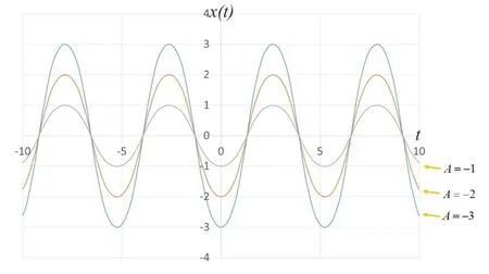
Figure 20: Wave obtained by the type(IV) exact solution at varying amplitude A(A=-1, -2, -3)

Figure 21: Wave obtained by the type (IV) exact solution at varying angular frequency ω

4.5 Numerical results of exact solution of type (V)

ForA=1, ω=1,andΦ=0in Eq. (3.18), the waves of the exact solution of type (V), leaf functionssleaf2(t)andcleaf2(t), and functionsare shown in Fig. 22. To show the wave of the type (V) exact solution, Fig. 23 shows an enlarged view of Fig. 22. The horizontal and vertical axes represent timetand displacementx(t), respectively. The numerical data of the type (V) exact solution can be obtained by using data given in Tabs. 5 and 7. To discuss the range ofx(t)in the type (V)exact solution, the following equation is transformed:

The following equation is obtained by squaring both sides of the above equation.

The sign of the first-order differential with respect to leaf functionssleaf2(t)andcleaf2(t)depends on domaintofx(t)(see Shinohara [Shinohara (2015)] or Eqs. (4.11) and (4.12)).The first-order differential of Eq. (4.51) is discussed by dividing the domain as shown in Fig.24.

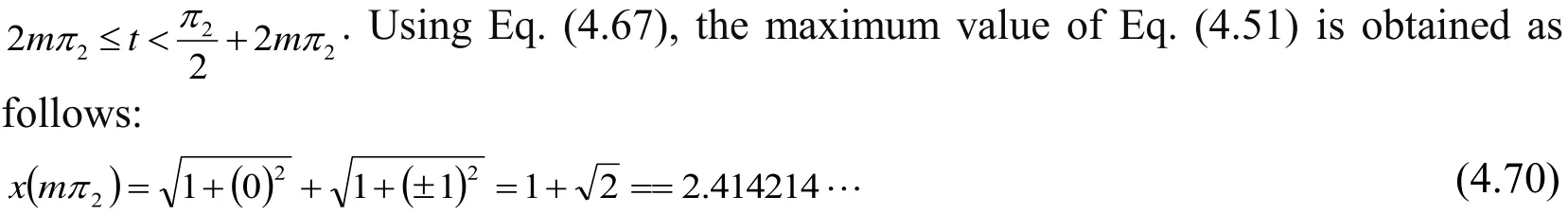
The extreme value of the type (V) exact solution is obtained bydx(t)/dt=0with Eqs.(4.52)-(4.55), as shown below.

Using Eqs. (4.57) and (B.1), the values of the leaf function are obtained. Form=2k(mandk: integer), the leaf function value is as follows:

Therefore,tdoes not satisfy condition (ii).

Next, we consider the case where condition (iii) is satisfied in Domain (1):

The centers of displacement and amplitude are

We now analyze Figs. 25 and 26. The variablesΦ=0andω=1are set, whereas amplitudeAis varied. Under these conditions, the waves obtained by the type (V) exact solution are shown in Fig. 25. The range of displacementx(t)can be obtained by the following inequality:

Next, the variablesΦ=0andA=1are set, whereas angular frequencyωis varied. The waves obtained by the type (V) exact solution are shown in Fig. 26. The period of the waves varies according to the absolute valueω; asωincreases, the period decreases. Forω=±1, the period becomes constantπ2/2, forω=±2, it isπ2/4, and forω=±3, it isπ2/6. By usingω, periodTis obtained as follows:

Figure 22: Waves obtained by the type (V) exact solution; leaf function and function

Figure 23: Enlargement of Fig. 22

Figure 24: Waves obtained by functions cleaf2(t), sleaf2(t), and -cleaf2(t)

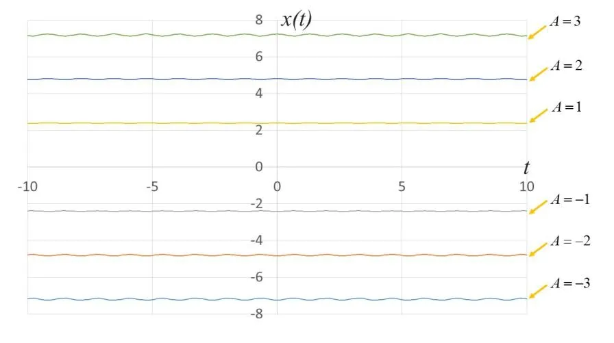
Figure 25: Waves obtained by the type (V) exact solution at varying amplitude A

Figure 26: Wave obtained by the type (V) exact solution at varying angular frequency ω

4.6 Numerical results of exact solution of type(Ⅵ)

ForA=1, ω=1,andΦ=0in Eq. (3.22), the waves of the exact solution of type (VI), leaf functionssleaf2(t)andcleaf2(t), and functionsshown in Fig. 27. The horizontal and vertical axes represent time and displacementx(t),respectively. The numerical data of the type (VI) solution can be obtained from the data given in Tabs. 5 and 7. To discuss the range ofx(t)inthe type (VI) exact solution, the following equation is transformed using leaf functionssleaf2(t)andcleaf2(t):

The above equation can be obtained by the same operation using Eqs. (4.46) -(4.51). To discuss the range ofx(t)in the type (VI) exact solution, the first-order differential is obtained. The sign of the first-order differential with respect to leaf functionssleaf2(t)andcleaf2(t)depends on domaintof variablex(t).The first-order differential of Eq. (4.83) is discussed by dividing the domains (1)-(4) as shown in Fig. 24.

The extreme value of the type (VI) solution is obtained bydx(t)/dt=0with Eqs. (4.84)-(4.87), which is the same equation as (4.56). Therefore, to satisfydx(t)/dt=0, it is necessary to satisfy any of the conditions (i)-(iii), as shown in Eqs. (4.57)-(4.59).

Domain (1): We consider the case where condition (i) is satisfied in Domain (1):

We now analyze Figs. 29-31. The variablesΦ=0andω=1are set, whereas amplitudeAis varied. Under these conditions, the waves obtained by the type (VI) exact solution are shown in Figs. 29 and 30. The range of displacementx(t)can be obtained by the following inequality:

The centers of displacementx(t)and amplitude are0.0and, respectively.

Next, the variablesΦ=0andA=1are set, whereas angular frequencyωis varied. The waves obtained by the type (VI) exact solution are shown in Fig. 31. The period of the waves vary according to the absolute valueω. Asωincreases, the period decreases. Forω=±1, the period becomes constantπ2, forω=±2, it isπ2/2, and forω=±3, it isπ2/3. By usingω, periodTis obtained as follows:

Figure 27: Waves obtained by the type (VI) exact solution; leaf function and function

Figure 28: Waves obtained by the type (VI) exact solution

Figure 29: Wave obtained by the type (VI) exact solution at varying amplitude A (A=-1,-2,-3)

Figure 30: Wave obtained by the type (VI) exact solution at varying amplitude A(A=1,2,3)

Figure 31: Wave obtained by the type (VI) exact solution at varying angular frequency ω

4.7 Numerical results of exact solution of type (VII)

ForA=1, ω=1,andΦ=0in Eq. (3.26), the waves of the exact solution of type (VII) and leaf functionssleaf2(t)andcleaf2(t)are shown in Fig. 32. The horizontal and vertical axes represent time and displacementx(t), respectively. The numerical data of the type (VII)solution can be obtained by using data given in Tab. 4. Next, the variablesΦ=0andω=1are set, whereas amplitudeAis varied. Under these conditions, the waves obtained by the type (VII) exact solution are shown in Figs. 33 and 34. To obtain the extreme values, the first-order differential is derived as follows:

The angular frequencyωis varied. The waves obtained by the type (VII) exact solution are shown in Figs. 35 and 36. As shown in the figures, periodTis obtained from angular frequencyωas follows:

Figure 33: Wave obtained by the type(VII) exact solution at varying amplitude A(A=1,2,3)

Figure 34: Wave obtained by the type(VII) exact solution at varying amplitude A(A=-1, -2, -3)

Figure 35: Wave obtained by the type (VII) exact solution at varying angular frequency ω (ω=1, 2, 3)

Figure 36: Wave obtained by the type (VII) exact solution at varying angular frequency ω (ω=-1, -2, -3)

5 Conclusions

By using leaf functions, the exact solution of the cubic Duffing equation can be derived under certain conditions. The waves obtained by the exact solutions are graphically visualized. The conclusions are summarized as follows:

・Through leaf functions, seven types of exact solutions can be derived from the cubic Duffing equation.

・The seven types of exact solutions have two parameters, namely, angular frequencyωand amplitudeA, which indicate the characteristics of the wave. The coefficients of the termsxandx3in the cubic Duffing equation can be described by both wave amplitudeAand wave frequency parameterωin the leaf functions. AmplitudeAof the wave becomes constant, even though these coefficients vary according to variation inω. In contrast,wave frequencyωof the wave becomes constant, even though these coefficients vary according to variation inA. Since parametersAandωdo not affect the characteristics of the wave, they are independent variables in the ordinary differential equation.

・As amplitudeAincreases (decreases), the height of the wave also increases (decreases).As the frequency parameterωincreases (decreases), the period of the waves decreases(increases). The waveform obtained by the nonlinear spring can be controlled by adjusting these variables. Several new waveforms satisfying the cubic Duffing equation can be constructed by combining both trigonometric functions and leaf functions.

In the future research, the relation between trigonometric functions and hyperbolic functions can be obtained by using imaginary numbers. The analogy also exists for leaf functions. These extended leaf functions are defined as hyperbolic leaf functions[Shinohara (2016)]. By using these hyperbolic leaf functions, leaf functions and exponential functions, we are able to derive more exact solutions of Duffing equation. It is in that future research that exact solutions can be presented.

Al-Jawary, M. A.; Al-Razaq, S. G.(2016): A SEMI Analytical iterative technique for solving duffing equations.International Journal of Pure and Apllied Mathematics, vol.108, pp. 871-885.

Belé ndez, A.; Belé ndez, T.; Martí nez, F. J.; Pascual, C.; Alvarez, M. L. et al.(2016)Exact solution for the unforced Duffing oscillator with cubic and quintic nonlinearities.Nonlinear Dynamics, vol. 86, pp. 1687-1700.

Chowdhury, M. S. H.; Hosen, M. A.; Ahmad, K.; Ali, M. Y.; Ismail, A. F.(2017):High-order approximate solutions of strongly nonlinear cubic-quintic Duffing oscillator based on the harmonic balance method.Results in Physics, vol. 7, pp. 3962-3967.

Cveticanin, L.(2013): Ninety years of Duffing’s equation.Theoretical and Applied Mechanics, vol. 40, pp. 49-63.

Dai, H.(2012): a simple collocation scheme for obtaining the periodic solutions of the Duffing equation, and its equivalence to the high dimensional harmonic balance method:Subharmonic oscillations.Computer Modeling in Engineering & Sciences, vol. 84, pp.459-497.

Elí as-Zú ñ iga, A.(2013): Exact solution of the cubic-quintic Duffing oscillator.Applied Mathematical Modelling, vol. 37, pp. 2574-2579.

Elí as-Zú ñ iga, A.(2014): Solution of the damped cubic-quintic Duffing oscillator by using Jacobi elliptic functions.Applied Mathematics and Computation, vol. 246, pp. 474-481.

El-Naggar, A. M.; Ismail, G.(2016): Analytical solution of strongly nonlinear Duffing oscillators.Alexandria Engineering Journal, vol. 55, pp. 1581-1585.

Euler, L.(1911): Leonhardi euleri opera omnia. Series I-IV A.Bassel: Birkhä user.

Fagnano, G. C.(1750): Produzioni matematiche del Conte Giulio Carlo di Fagnano.Pesaro: Gavelli. Feigenbaum, L.(1981):Brook Taylor’s Methodus Incrementorum: A Translation With Mathematical and Historical Commentary(Ph.D Thesis).Yale University, New Haven.

Ganji, S. S.; Barari, A.; Karimpour, S.; Domairry, G.(2012): Motion of a rigid rod rocking back and forth and cubic-quintic Duffing oscillators.Journal of Theoretical and Applied Mechanics, vol. 50, pp. 215-229.

Hosen, M. A.; Chowdhury, M. S. H.(2016): Solution of cubic-quintic Duffing oscillators using harmonic balance method.Malaysian Journal of Mathematical Sciences,vol. 10, pp. 181-192.

Kovacic, I.; Brennan, M. J.(2011):The Duffing equation: Nonlinear oscillators and their behaviour. John Wiley & Sons, USA.

Liao, H.(2014): Nonlinear dynamics of Duffing oscillator with time delayed term.Computer Modeling in Engineering & Sciences, vol. 103, pp. 155-187.

Liu, C. S.(2014): Disclosing the complexity of nonlinear ship rolling and Duffing oscillators by a signum function.Computer Modeling in Engineering & Sciences, vol. 98,pp. 375-407.

Ranjan, R.(2017):Elliptic and Modular Functions from Gauss to Dedekind to Hecke.Cambridge University Press.

Sayevand, K.; Baleanu, D.; Fardi, M.(2014): A perturbative analysis of nonlinear cubic-quintic Duffing oscillators.Proceedings of the Romanian Academy Series AMathematics Physics Technical Sciences Information Science, vol. 15, pp. 228-234.

Shinohara, K.(2015): Special function: Leaf functionr=cleafn(l)(Second report).Bulletin of Daido University, vol. 51, pp. 39-68.

Shinohara, K.(2015): Special function: Leaf functionr=sleafn(l)(First report).Bulletin of Daido University, vol. 51, pp. 23-38.

Shinohara, K.(2016): Special function: Hyperbolic Leaf functionr=sleafhn(l)(First report).Bulletin of Daido University, vol. 52, pp. 65-81.

Shinohara, K.(2016): Special function: Hyperbolic Leaf functionr=cleafhn(l)(Second report).Bulletin of Daido University, vol. 52, pp. 83-105.

Shinohara, K.(2017): Addition formulas of leaf functions according to integral root of polynomial based on analogies of inverse trigonometric functions and inverse lemniscate functions.Applied Mathematical Sciences, vol. 11, pp. 2561-2577.

Sibanda, P.; Khidir, A.(2011): A new modification of the HPM for the Duffing equation with cubic nonlinearity.Proceedings of the 2011 international conference on Applied & computational mathematics, pp. 139-143.

Zhang, Y.; Du, L.; Yue, X.; Han, Q.; Fang, T.(2015): Analysis of symmetry breaking bifurcation in Duffing system with random parameter.Computer Modeling in Engineering& Sciences, vol. 106, pp. 37-51.