Feng HE,Ershuai LI

School of Electronic and Information Engineering,Beihang University,Beijing 100083,China

Deterministic bound for avionics switched networks according to networking features using network calculus

Feng HE*,Ershuai LI

School of Electronic and Information Engineering,Beihang University,Beijing 100083,China

Deterministic bound; Grouping ability; Network calculus; Networking features; Switched networks

The state of the art avionics system adopts switched networks for airborne communications.A major concern in the design of the networks is the end-to-end guarantee ability.Analytic methods have been developed to compute the worst-case delays according to the detailed con figurations of flows and networks within avionics context,such as network calculus and trajectory approach.It still lacks a relevant method to make a rapid performance estimation according to some typically switched networking features,such as networking scale,bandwidth utilization and average flow rate.The goal of this paper is to establish a deterministic upper bound analysis method by using these networking features instead of the complete network con figurations.Two deterministic upper bounds are proposed from network calculus perspective:one is for a basic estimation,and another just shows the bene fits from grouping strategy.Besides,a mathematic expression for grouping ability is established based on the concept of network connecting degree,which illustrates the possibly minimal grouping bene fit.For a fully connected network with 4 switches and 12 end systems,the grouping ability coming from grouping strategy is 15–20%,which just coincides with the statistical data(18–22%)from the actual grouping advantage.Compared with the complete network calculus analysis method for individual flows,the effectiveness of the two deterministic upper bounds is no less than 38%even with remarkably varied packet lengths.Finally,the paper illustrates the design process for an industrial Avionics Full DupleX switched Ethernet(AFDX)networking case according to the two deterministic upper bounds and shows that a better control for network connecting,when designing a switched network,can improve the worst-case delays dramatically.

1.Introduction

The embedded avionics system is a typical mission-critical and safety-critical system.During the past several decades,it has evolved from a federative architecture where calculators and

Nomenclature

actuators were interconnected through dedicated monoemitter links(such as ARINC 429)towards an Integrated Modular Avionics(IMA)architecture in which switched fabrics are adopted for airborne communications.1,2IMA platform can be seen as a set of modules,switches and links.Because of their critical natures,IMA platform must satisfy strong real-time requirements,such as latency and jitter,and this kind of requirements are also reflected into the embedded network which constitutes the basic infrastructure for airborne communications.What’s more,it should provide the guarantee ability for the Worst-Case(WC)delay control.

There are several networking solutions for IMA communications.Among these methods,ARINC 664 part 7 technology,3commonly called AFDX (Avionics Full Duple X switched Ethernet),is one of the most successful solutions and becomes the de facto standard in the context of avionics communications.AFDX is a switched Ethernet technology and takes into account avionics constraints.All flows in AFDX are asynchronous,but have to respect a bandwidth envelope(burst and rate)by Virtual Links(VL).For a given flow,the end-to-end delay of a packet is the sum of transmission delays on links and queuing latencies in output ports,and the latter contribute the main uncertainty during transmission.Therefore,it is important to perform a deterministic latency analysis in each output port.For certification reasons,there are several methods to compute the delays,such as Network Calculus(NC),4–6Trajectory Approach(TA),7–9and Holistic Method(HM).10All of these methods need detailed network con figurations,such as network topology,each flow’s period,payload,and routing paths.

In the early stage of an IMA system design,it is in great need to make a general performance prediction before network being implemented in detail.1During this stage,a system designer may only have some general pro files about the embedded switched network,such as the overall bandwidth utilization rate,network scale,and the average rate for flows.It is obliged to predict a deterministic delay bound according to these general switched networking features,and then the system designer can use this bound to restrict the network scale, flows count,and bandwidth utilizations to assure an overall system performance guarantee.At the same time,it is also meaningful to make a rapid network performance assessment from an overall aspect after the embedded network has been constructed,and this overall performance also provides a certain kind of network certification from the global perspective.

Focused on a Guaranteed Rate(GR)network,11such as Differentiated Services(DS),there are some deterministic bounds restricted by a set of general networking features.11,12The simplest bound is related with flow hops,utilization,and scaled burst.If the detailed local scheduling strategy is considered,an improved bound of delays can be obtained.Unfortunately,these bounds cannot cope with AFDX-like networks or some other switched solutions(such as Fibre Channel(FC))due to the fact that AFDX-like networks cannot provide such kind of GR services.Considering the flow envelop process by VL,it is only a shaping method for flows and cannot ensure that every flow could be forwarded at a given server rate in each output port.

This paper deals with a novel approach for rapid network delay bound estimation within the avionics context according to some switched networking features from network calculus perspective.13According to its theory,input flows and output ports are respectively modelled with traffic envelopes and service curves,and these elements can be abstracted into some more general switched features easier than trajectory approach8or Model Checking(MC).14,15Since network calculus approach has been improved by adding a grouping technique9in the context of AFDX,we will also make a further discuss on the bene fit from group strategy and figure out the possible benefit range.

The paper is organized as follows.After a short introduction about the related work in Section 2,we focus on the upper bound model ling based on a set of switched networking features for the worst-case delay analysis in Sections 3 and 4.Further discussion about the measurement of grouping benefit is carried out in Section 5.A fully connected network and an industrial AFDX networking case are used to illustrate our approach in Section 6,where some discussions are included.Finally,conclusions are presented in Section 7.

2.Related work

The analysis of end-to-end delays within embedded networking contexts has been addressed in literatures.Classically,end-to-end delays are computed based on network calculus4,5,16–18theory by using(min,plus)operations,13which has been successfully applied to AFDX.It models the coming flows with upper envelopes and service abilities with lower envelopes,and changes the uncertain degree of flow’s arrival into flow’s maximal burst.Therefore inevitably,it will bring some pessimism for delays evaluation.Much work has been done to tighten the upper bound.The most remarkable improvement is related to a grouping strategy,18or serialization effect.In particular,Bauer et al.9gave the average group benefit as 24.21%for an industrial AFDX network with more than 1000 VLs.Besides the deterministic versions of network calculus,stochastic versions6also have been studied for avionics network by mixing the basic model with larger deviation theory,which can perform the end-to-end delay estimation under a given confidence probability.19This kind of work based on network calculus can further be found for different networking solutions,such as TTEthernet20and Ethernet-AVB(Audio Video Bridging).21,22

The second analysis method for end-to-end delay computing is related to trajectory approach.7–9,23The basic idea of trajectory approach is to identify the busy period for a packet when it suffers the worst-case blocking along its paths.Since grouping strategy has been used to improve the end-to-end delay upper bound for network calculus,it also has been considered for trajectory approach and the average grouping bene fit is 18.36%.9Still there exist some inherent pessimism,such as the overestimation of competing workload,double counting frame with the maximal packet length and the underestimation of serialization effect.24Further revisited version can be found in Ref.23Compared with network calculus with grouping strategy,trajectory approach with grouping can achieve 10%9better tightness in average for the end-to-end delay estimation.The state of art of trajectory approach has been implemented for Ethernet-AVB.25

Both network calculus and trajectory approach are approximation methods for the upper bound.Thus,some exact worst-case delay analysis methods have been developed,such as model checking14,15approach.However,it cannot cope with real avionics networks due to the combinatorial explosion problem for large con figurations.Simulation method16,26,27can manage delay estimation for real avionics networks,especially from the average delay aspect.But its results cannot be used to represent the worst-case performance of the target network due to the missing of some rare events,which maybe lead to underestimation of the real upper bound.Also,the precision of simulation depends on the correctness and effectiveness of the corresponding simulation model.

Besides the approaches mentioned above,there are some other analysis methods.Holistic method10is a composable response time analysis method taking into account input offsets and jitters of flows.It investigates the best-case and worst-case delays in each forwarding node along flow paths,and then these results are assembled together to constitute the final delays.Though holistic method should be pessimistic,it has a fast analysis speed.10Forward end-to-end delays Analysis(FA)28is based on real-time scheduling and considers the problem of node with high load(over 100%).Focusing on this problem,FA can still achieve a reasonable computing result,in spite of some pessimism,in contrast to computing failure for trajectory approach.Also there exist some other analysis methods like queuing theory29with M/M/1 model.Although queuing theory has widely been applied to the average performance evaluation for consumer-service models,it still does not suit avionics environment due to the lack of worst-case consideration.

All of the above methods depend on the detailed con figurations about flows and networks.In fact,the requirement of a fast upper bound estimation for embedded networks according to some typical networking features has been concerned in literatures.Nesrine et al.2treated the delay of flows in the embedded network as a time interval with one upper bound and one lower bound brie fly.Nam et al.1,30analysed the delays in a specific switched network by assuming that flows could be served at most in two clock periods.Thus,the final delays of flows can be guaranteed with a simple upper bound expression.To some extent,the scheduling strategy in Ref.30is also one kind of guaranteed rate scheduling method since it can ensure a deterministic delay limit of no more than two clock periods for any feasible flow.Besides,there are two other methods to measure the upper bound for guaranteed rate networks:one is for a basic condition with flow hops,utilization,and scaled burst;the other considers the local scheduling strategy adopting Static Earliest Time First(SETF).However,these upper bounds do not suit switched networks like AFDX and FC.Considering flow shaping process by a VL in AFDX,it cannot ensure an interval[an,fn+e]in which every packet belonging to the VL can be forwarded successfully,where anis the arrival time for the nth packet;e is a fixed delay(such as technology delay);fnis the departure time of the packet and should satisfy:

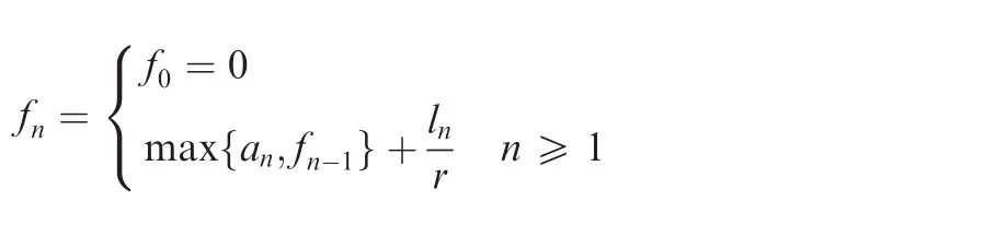
where lnis packet length and r is GR node server rate.

This paper deals with a novel analytic method for the end to-end delay estimation according to some typically switched networking features instead of the detailed con figurations.It investigates the problem how we can achieve a deterministic upper bound for a switched network if we have no detailed con figurations only with these typical features and some general pro files.The problem is shown in Fig.1.

The first contribution of this paper is to present two deterministic upper bounds for the worst-case end-to-end delay estimation for switched networks without detailed flow and network information,such as routing tables,topology and connecting information, flow con figurations and scheduling methods.

The second contribution of this paper deals with the explanation of how grouping strategy plays a role in the final end to-end delays from system aspect instead of individual flows,and the measurement model of the possibly minimal grouping benefit from grouping strategy according to network connecting degree.

The third contribution of this paper is to provide an analysis of the possibly maximal network utilization according to our deterministic upper bound.

3.Basic deterministic upper bound

3.1.Typical networking features

When we consider the periodicity of avionics applications,most flows in the IMA platform obey the leaky bucket model,which can be described by two typical parameters:period(or the minimal packet interval)and payload.Thus,a common avionics switched network,like AFDX,can be abstracted into some general switched features,11and these features will further be conducted to obtain our deterministic bounds.

C:link speed.Without loss of generality,the speeds of all physic links are supposed to be the same within the whole embedded network,such as C=100 Mbit·s-1.

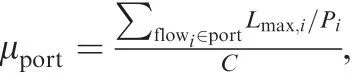
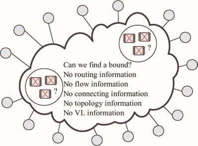
Fig.1 Problem of computing deterministic bound only with some switched networking features.

For a practical network,the traffic’s arrival may not obey the strict period restriction and might have varied packet lengths.However,typically it should have a minimal packet interval and a permitted maximal packet length especially in avionics context.For certification reason,parameters(Lmax，i,Pi)can be used to stand for the largest bandwidth requirement.

ρ: flow constant bit rate.First,ρ is de fined as a uniform flow constant bit rate.It means that each flow has the same bit rate as Lmax/P within the whole network.This assumption is quite arbitrary for a real industrial network.Later,we will discuss how to weaken this assumption.In fact,ρ can be the minimal average flow constant bit rate among all output ports in ESs and switches.In another word,it can beandis the average bit rate of flows in a specified portj.

l:upper limit of packet length.Each flow has its own packet length Lmax,and the maximal packet length among all flows within the whole network is l,soalso can be a constraint for all flows de fined by system designers during the first design stage.

h: flow hop.h is the count of flow hops when it crosses switches according to its routing path.So for a given flowi,it has its own flow hop asThe maximal hop number among all flows within the whole network isLike parameters μ and l,h also can be a constraint for all flows to restrict the scale of the whole network.

3.2.Latency at source node

Flow interference starts at the source node,which is shown in Fig.2.There are multiple flows generated at the same source node.Limited by the physical speed of the output port,all of these flows attend the competition to be scheduled out under a certain scheduling strategy,such as First In First Out(FIFO).Considering the worst-case scheduling scenario,the maximal blocking for a given flow takes place under the following two conditions:(A)The considered flow and all the other flows’packets arrive at the buffer at the same time;(B)The considered flow packet has to wait until all the other flows’packets finish their transmission and then it can get the chance to be scheduled out.

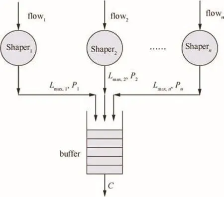
Fig.2 Flow latency analysis at source node.

Under this assumption,the worst-case latency for any given flowiat the source node is bounded by

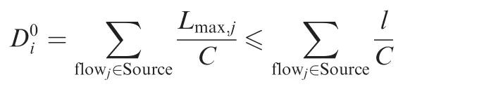
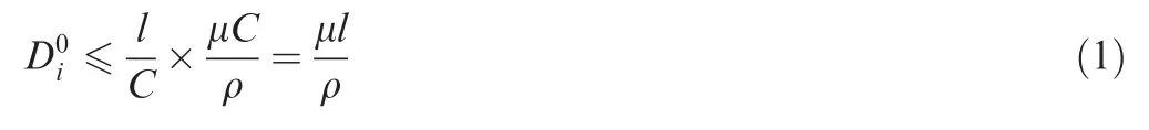
Since each flow has the same constant bit rate ρ and the maximal bandwidth utilization rate is μ,the number of flows at the source node is no more than n= μC/ρ.Then the worst-case latency at the source nodecan be changed into

For the follow-up analysis,NC should be used to establish flow’s model in the following switch nodes.The basic concept of NC can be found in Appendix A.According to its theory,when a flow R(t)is just scheduled out from an output port,its equal departure burst will become fuzzier and larger and this kind of burst enlargement can lead to a further uncertainty of flow’s arrival in the following switches.When considering the departure curve of flowiafter the source,it will have a bigger burst toleranceaccording to NC:16

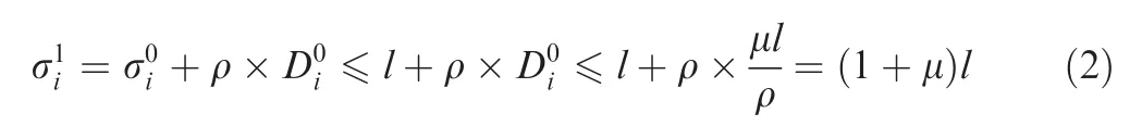
In Eq.(2), flow’s constant bit rate ρ is neutralized by delayand the enlarged departure burst is limited by bandwidth utilization rate μ and packet maximal length l.This equivalent output flow model can be used for the latency analysis at the following switch nodes.

3.3.Latency at switch nodes

In order to compute the end-to-end delay of a flow,the whole scheduling and transmitting process along flow’s path should be investigated.But in our model,there is no detailed information about flow’s path,so some alternative methods should be used to make up the lack of the corresponding path information.Typically,it should consider switched features and also should guarantee the worst-case blocking estimation.

Considering flow forwarding behaviour in the following switch nodes, flow interference also exists and these aggregated flows may come along different paths as shown in Fig.3.Taking flow1(in Fig.3)for example,the interfering flows may come from other source nodes( flow2),from one-hop switch( flow3),two-hop switches( flow4),even up to(h-1)hop switches( flow5).For the considering flow1,the worst-case blocking scenario should be figured out in its forwarding switches,such as in S1and S2.

Obviously,the worst-case blocking takes place under the condition that all the other interference flows come from their possibly maximal switch hops to lead to the corresponding biggest bursts,as well as the maximal uncertainty of arrivals.In Section 3.1,we have made an assumption that the maximal flow hop is no more than h throughout the whole network,so the maximal number of hops for these interference flows before they enter into switch S1(see Fig.3)is bounded by(h-1).During the previous(h-1)switches,these interference flows may experience a variety of blocking from any other flow sharing the same paths,and finally these interference flows obtain their biggest equivalent bursts to bring the most serious blocking effects to the considering flow1.

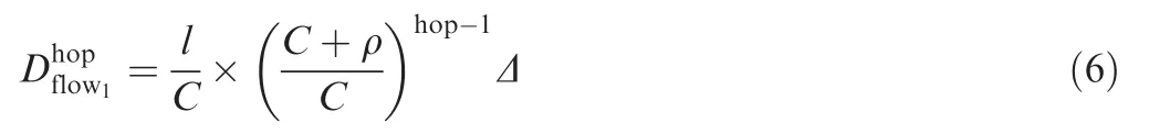
In order to find out the equivalent burstof the arrival curve in the(hop)th switch(or the equivalent departure burst for the output curve after the(hop-1)th switch),the burst tolerance is supposed to be limited by packet maximal length Lmaxand an enveloping function f′(hop，i)with the actual flow hop as the dependent variable,and f(hop)is used to stand for the upper bound of all f′(hop，i)functions.

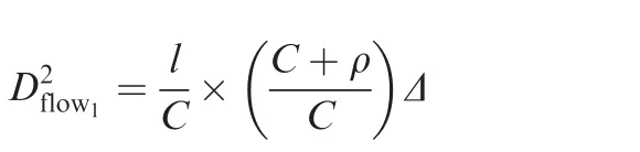
For the considered flow1,its equivalent arrival burst in the first switch S1isaccording to Eq.(2),so the worst-case latency for flow1in S1is

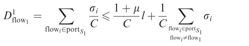
Since flows can obtain bigger burst tolerances when they experience more switches,the other interference flows’burst tolerances must be less than the upper bound of burst after(h-1)switches as they have just entered the last switch.Then,the blocking by other interference flows to the considered flow1is bounded by

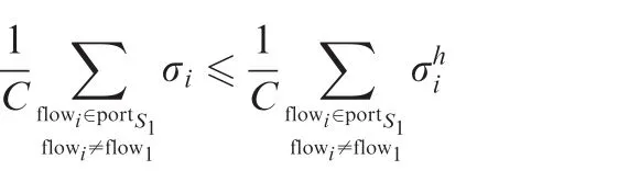
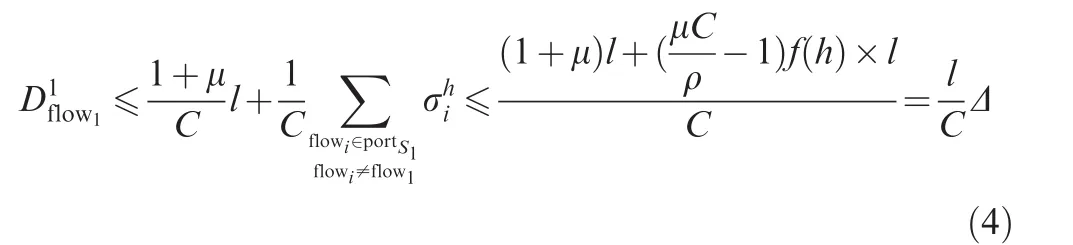
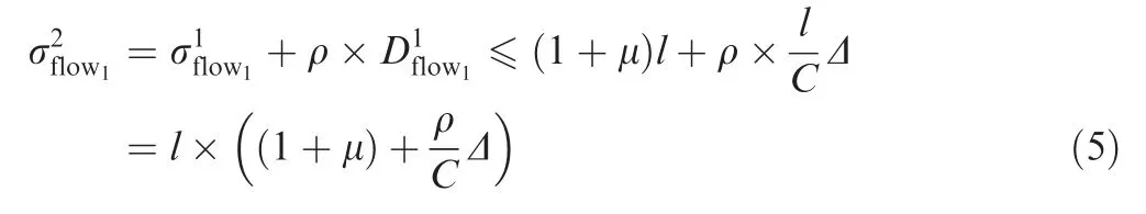
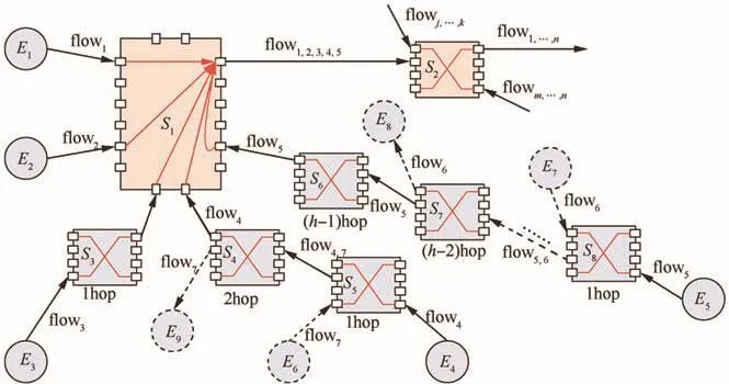
Fig.3 Flow latency analysis at switch nodes.

and the departure burst of flow1after the second switch S2is bounded by

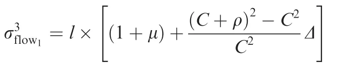
Adopting the same analysis method,further results for latencies and equivalent arrival bursts can be obtained.In fact,for flow1,its latency at(hop)th switch has a closed form as

and the closed form for the equivalent arrival burst at the(hop)th switch can also be deduced as

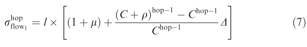
Since flow1is randomly selected out from the switched network,for any flowi,its(hop)th latency and equivalent arrival burst still obey the restrictions shown in Eqs.(6)and(7).

Combining Eqs.(3)and(7),we can get the detailed expression for f(hop=h)function,which is typically de fined by h:

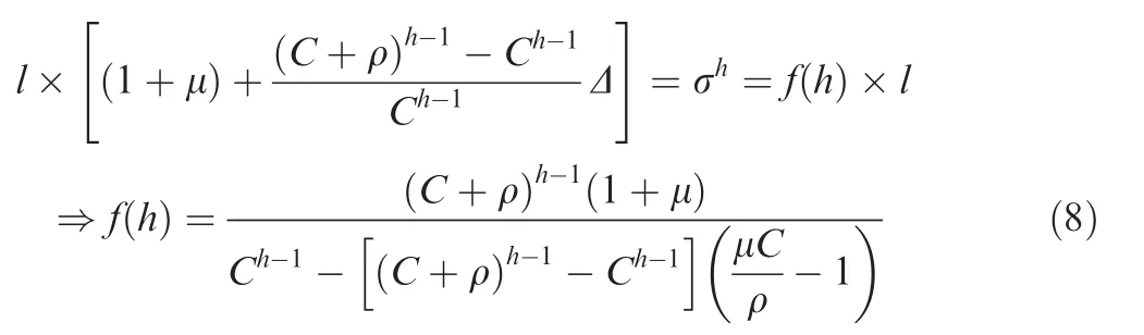
Let h=0,and we will get f(0)=1 according to Eq.(8),which means that the original burst of flows is no more than f(0)×l=l,and then we can find that Eq.(8)is also suitable for the source burst analysis.

3.4.End-to-End delay bound

In Section 3.3,we obtained the closed forms for flow’s arrival burst and latency at(hop)th switch.These expressions are based on Δ as well as f(h).

For the end-to-end delay,the latencies at the source node and switch nodes according to flow’s routing paths should be added together to constitute the final result.Since flow’s hop cannot exceed h,the final delay can be calculated by

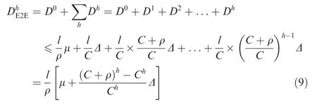
Though delay D0at the source node is added into Eq.(9)separately to constitute the end-to-end delay bound,the final expression is still reasonable when h=0,which means that there is no switch in the network and the communication model is just a point-to-point style.Thus,for Eq.(9),the range of h can bewheres the natural number set.

4.Deterministic upper bound with grouping strategy

In this section,the effectiveness of grouping strategy on flow deterministic bound will be discussed and illustrated.According to network calculus theory,grouping strategy can dramatically decrease the pessimism of the end-to-end delay analysis especially when a large number of flows share the same paths.Since these grouped flows will keep their queuing sequences when they enter the next switch,the grouped flows can be treated as an integrated flow from the merged node to the first separated node,and the individual burst of every flow in the integrated group can be wiped out but only with one burst to stand for the whole group.This kind of queuing behaviour also reflects the philosophy of Pay Burst Only Once(PBOO).

Grouping strategy can be illustrated in Fig.4.There are two grouped flows( flow2, flow3)and( flow6, flow9)and one simple flow( flow4)aggregating in the same output port(14，S1)in switch S1.Strictly speaking, flow4can also be seen as a group but just only with one flow in it.

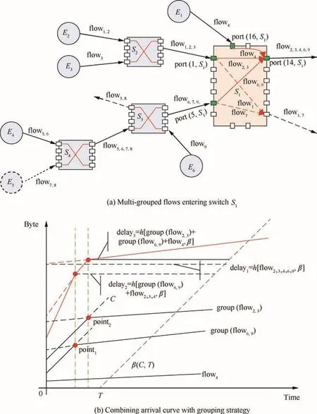
Fig.4 Flow group analysis at switch nodes.

Focused on these grouped flows,all the key points in the arrival curves(point1and point2for example in Fig.4(b))should be figured out first.Group( flow2,3)comes from port(1，S1)and the flows in this group have been serialized by switch S2before they enter into switch S1,which will lead to one inflection point2in the corresponding arrival curve.The same is for group( flow6,9).Thus,the combining arrival curve at port(14，S1)should have two inflection points and three piecewise slopes.Different in flection points determine different latency results.If all the benefits coming from grouping strategy are counted on,the tightest result for the worst-case latency analysis can be achieved.For example,delay3according to the last inflection point will be much tighter than delay1and delay2since delay3thinks of all of the grouped flows.The service curve in Fig.4(b)is considered as the rate-latency model with C as the service rate and T as the maximal technology latency.More detailed information can be found in Appendix A.

4.1.Parameters for grouping feature

Besides the parameters de fined in Section 3.1,some new parameters are needed to describe grouping features.

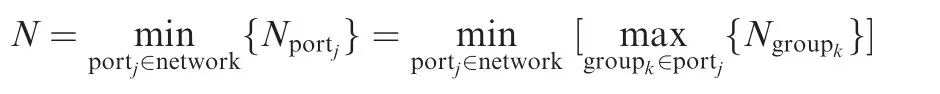
N:group capacity.In each group,two or more flows are serialized.The count of flows in a group is de fined as group capacityIn an actual output port,there may be several groups coming from different previous nodes,and the maximal group capacity among all of these groups in the same output port can be selected out as Nport=maxgroupj∈port｛Ngroupj｝.From a global aspect of the whole network,the minimal value of all Nportis N.

According to the definition of N,it just reflects the capacity of grouping in a switched network.If there is no grouped flow at least in one output port,then Nport=1,which furthermore results in N=1.Later,a further discussion about N will be made to increase the flexibility to measure group benefit.

4.2.Delay bound with grouping strategy

In order to calculate the influence from group strategy, first it needs a way to compute all the inflection points in the combining grouped arrival curve.Aimed at each group,its arrival curve can be described by a VBR model(bM,p,r,b)which means that the arrival curve obeys α(t)=min(bM+p × t，b+r×t)(t≥0).11According to VBR model,the in flection point isSince every group is serialized by physical links,the corresponding parameters in our model can be more explicit asandAdopting the same way in Section 3.3 for the consideration about flow’s burst and its hop,we still suppose that the burst tolerance of a flow in the(hop)th switch is a function of the upper limit packet length l and the actual hop number,which can be written as σhop≤ fg(hop)×l.Thus,bMshould be fg(hop)×l since it is the maximal flow burst among the grouped flows.Parameter b also has an explicit expression as b=Ngroup×fg(hop)×l.According to these specific parameters,the in flection pointfor a grouping model can be obtained.

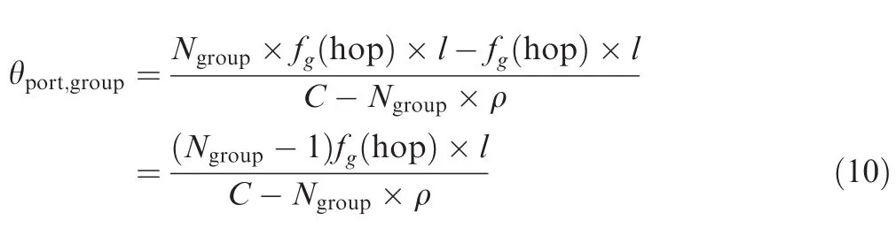
In order to obtain the grouping delay,it is necessary to figure out which key point should be taken out as the referenced point among all the key points in the combining arrival curve for the group.According to Eq.(10),it is clear that θport，groupis an increasing function byand fg(hop).A larger Ngroupor fg(hop)will bring a biggerwhich finally will result in a tighter latency bound according to Fig.4.Focused on an actual output port,the last inflection point in the arrival curve determines the tightest delay bound.In order to find this bound,all θport，groupshould be compared to select out the maximal one.As Nportis the biggest value of all Ngroupin the considered port,Nportcan be used to replace Ngroupto compute the last inflection point.From the global networking aspect,a more general expression should be found for the selection about the last point.Though the maximal one among all Nportcan be used for a better bound result,it also means that there are some other ports which cannot achieve to this grouping degree and maybe results in an optimistic estimation.But if the minimal one among all Nportis selected out for the following analysis,a more general and proper expression for the effectiveness evaluation of grouping strategy can be obtained,though there are some losses of tightness.

Furthermore,although N can be used to replace Ngroupfor generality,the inflection point θport，groupis still related to fg(hop),which will bring great complexity to calculation of a general expression for this inflection point.Considering an actual output port,there may be several groups and these grouped flows may come from different previous nodes.The flow with the biggest burst among all the flows must experience the most switches and will count on bM.For the sake of convenience,the biggest burst flow is selected out and supposed to have a corresponding index as jM.For the other flows in the same group except flowjM,the hypothesis that all these flows just come from their source is a safe condition to avoid an optimistic estimation about the last inflection point.Since flow burst σhopis an increasing function by flow hop number according to Eqs.(3)and(8),we have

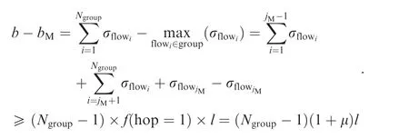
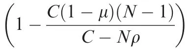
Thus,a more general expression for the last inflection point from the global perspective can be obtained if N is used to replace Ngroup:

Adopting the similar analysis method in Section 3.3,the latencies at switch output ports should be analysed from upstream to downstream.For a considered flowiwhich is just transmitted out from its source node and enters its first switch output port,the accumulated flow bits for all flows at the last inflection point at this port should be

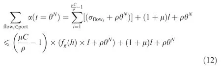
In Eq.(12),the bursts of all other interference flows are still supposed to achieve the upper bound as fg(hop=h)×l to cause the worst-case blocking.Thus,the latency at the first hop switch for the considered flowiis

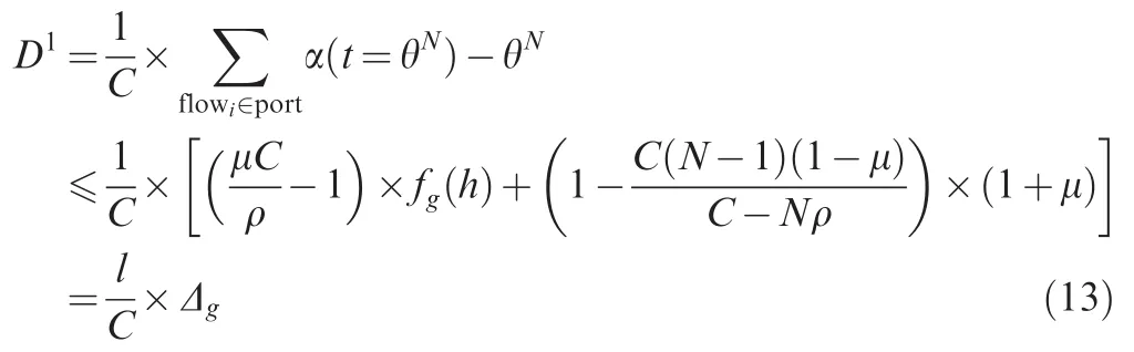
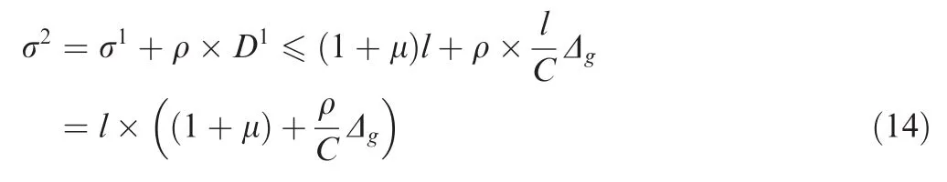
The following deducing process is similar as what is shown in Sections 3.3 and 3.4.By using the mathematical induction method,the closed forms for latency,burst tolerance and end-to-end delaywith grouping can be obtained.In fact,these expressions look quite similar as Eqs.(6),(7)and(9)except the different definitions of Dgand fg(h).

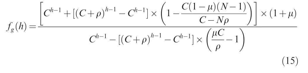
According to Eq.(15),fg(h)will have the same expression as f(h)if N is set to 1,which means that fg(h)is also suitable for the condition that grouping strategy is not applied to the end-to-end delay calculus.Besides,letting N=1 will also lead to the same expression of the end-to-end delay with grouping strategy as the expression without grouping shown in Eq.(9).It is reasonable because the condition of N=1 just means that there is no grouping flow in the whole switched network or at least in some output ports,in another word,the flow grouping is not a common phenomenon throughout the whole network,and then the advantage of grouping is close to zero.

4.3.Discussion on constant bit rate

In Section 3.1,we have given the definition of parameter ρ as a uniform flow constant bit rate for all flows in the whole network.In this section,a further discussion will be performed and a more general concept for it will be given.

As an important role in the end-to-end delay analysis,the value of ρ (together with μ)determines the number of flows taking part in the aggregating behaviour.When μ is fixed,the smaller ρ is,the more flows there would be in the considered port,which will result in a bigger latency finally.

Considering an actual output port,the aggregating flows may have different constant bit rates according to their different flow con figurations as ρflowi=Lmax，i/Pi.The average constant bit rate in this port should be

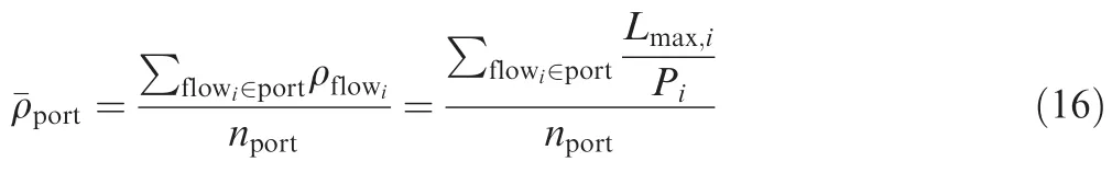
It just shows that the counts of flows are the same for both average¯ρ condition and uniform ρ condition if the average constant bit rate¯ρ in an actual output port is equal to the uniform flow constant bit rate ρ.Thus,the worst-case latency for average¯ρ will be no worse than the uniform ρ assumption.Therefore,a more general definition for ρ could be the average constant bit rate as shown in Eq.(16).

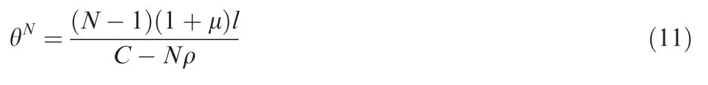
5.Grouping ability analysis

In Section 4.1,the concept of N which means group capacity has been de fined.In fact,N is not so easy to be figured out by architecture designers.In this section,a more flexible and measurable model for it will be discussed and an alternative parameter will be given,which also reflects the nature of switched networking features.What’s more,it can be used to measure the grouping ability for a switched network.

Deg:network connecting degree.Focused on any node in a switched network,the parameter Degnodeis used to measure its connecting degree.From the global perspective,the maximum of all Degnodeis de fined asSo Deg just reflects the connectivity ability for a switched network.

The concept of Deg can be further illustrated in Fig.5.For switch S1,it has been connected with different nodes,such as the source nodes E1,E2,E3and switch nodes S2,S3,S4,and thus its connecting degree is DegS1=6.

Considering one output port in S1,such as port(14，S1)who connects with E3,the aggregated flows coming from different connecting nodes constitute different flow groups.Aimed at one flow in a group,no matter how many hops it has experienced,the considered flow with the other flows in the same group has just been serialized by a common previous port.For example,every flow in the group set( flow3,1,...,flow3，n3)must be serialized by a specific port in switch S2.From the perspective of network connectivity,each output port might receive the coming flows from all of the connecting nodes except its own,especially when the distribution of flows within the whole network follows an even mode.

By using the concept of Deg,a more flexible and measureable model for group capacity N can be established based on the assumption that the dispatchment of flows throughout the whole network obeys a uniform distribution,not only for the residence of sources and destinations but also for the routing of flows.

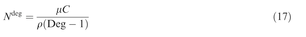
Focused on an actual output port,the distribution of flow bit rates cannot obey the uniform mode in most cases,and an equal expression for the estimation of the average group capacity can also be de fined as

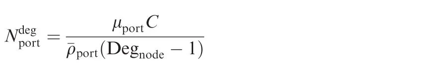
Since some groups in a practical output port may contain more flows than the average level and some may have less,the value of Nportshould be no less than the value ofasis the maximum value of all group capacities in the considered port.Thus,ifis used to calculate the end-to-end bound with grouping strategy instead of Nport,the result will be more pessimistic.But the concepts of N and NDegare still quite different.If the distribution of flows is so ragged that there is no grouped flow at least in one port throughout the whole network,the original group capacity can be N=1;however the new definition of group capacity according to Eq.(17)may be bigger than 1.Thus,NDegcan be seen as a reference for N.In most cases,the adopting of NDegwill get a more pessimistic estimation.But NDegis still useful especially for architecture designers who maybe have no idea about the specific group capacity during the stage of design but might have a basic design philosophy for network connecting degree.

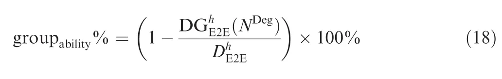
In fact,NDeghas a more important usage than the reference for N.It can be used to measure the grouping ability from grouping strategy since it just reflects the minimal possibility that the end-to-end bound can be improved by grouping features in switched networks.

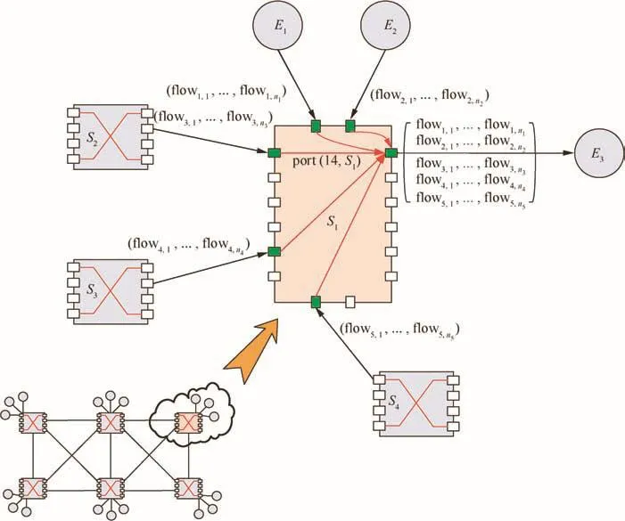
Fig.5 Network connecting degree for switch S1.

6.Case study and comparisons

6.1.GR bound comparison

In this section,our basic deterministic bound DE2Ewill be compared with two typical GR bounds:one is a basic GR model and the other is an improved GR model.

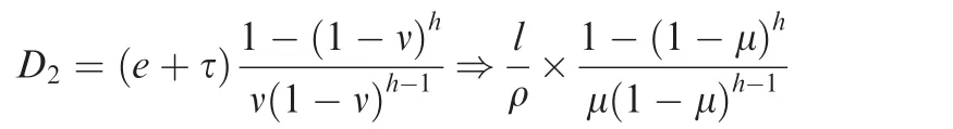
Bound 1.11Considering a differentiated service,if each node in the backbone network can provide a GR guarantee,the upper bound of delay is

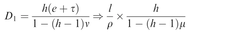
The definition of v in the Ref.11is utilization factor,which has the same meaning as μ.e and τ in the Ref.11are latency and scaled burstiness factor,which can be replaced by l/ρ according to our model.

Bound 2(improved model).12Considering a differentiated service with Static Earliest Time First(SETF)scheduling strategy,the upper bound of delay can be improved as

The following comparisons are based on some typical network parameters,such as l=1000 bytes and C=100 Mbit·s-1.The results are shown in Fig.6(delay contours)and the numbers along the contour lines are the corresponding delay bounds.Both in Fig.6(a)and(b),the red lines stand for our basic bound model DE2E,the black lines stand for D1bound,and the blue lines stand for D2bound.The unit of delay bounds is ms.

From Fig.6(a),we can find:if the maximal hop is fixed as 3,our basic bound model DE2Ewill obtain a better estimation for the final end-to-end delay upper bound than the two GR models when bandwidth utilization rate μ within the whole network is set to a relatively small value(DE2Ehas a bigger contour range under a given delay bound value than the two GR models).But if μ is set with a relatively big utilization rate(such as more than 0.5),the improved GR model bound D2can achieve a better result.It can be explained since GR servers can ensure a guaranteed service rate for flow’s forwarding under any aggregating circumstance,but our model has no such a scheduling ability.It just assumes that all flows’asynchronous arrival at the output port causes the worst-case scheduling schema.Thus,the upper bound difference between our basic model DE2Eand the improved GR model D2for large value of μ originates in the unfair flow scheduling strategy.However,our bound is still better than the basic GR model D1when μ is assigned with a big value.Fig.6(b)just shows the influence of h and μ when ρ is fixed as 0.1 Mbit·s-1.In most cases,our model DE2Eachieves better than the two GR models since it covers a bigger region under a given contour value.

6.2.Maximal reachable boundary

Besides the comparisons mentioned in Section 6.1,the results in Fig.6(especially in Fig.6(a))also show that there are some unreachable areas of the upper bound not only for our basic model but also for the given GR models especially when network utilization rate μ or hop h is assigned with large values.

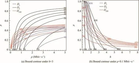
Fig.6 Bound comparison with GR models(delay contour).

The edges of these unreachable areas can be seen as the maximal reachable boundaries.According to Eqs.(9)and(8),the boundary can be obtained directly by setting the denominator to zero:

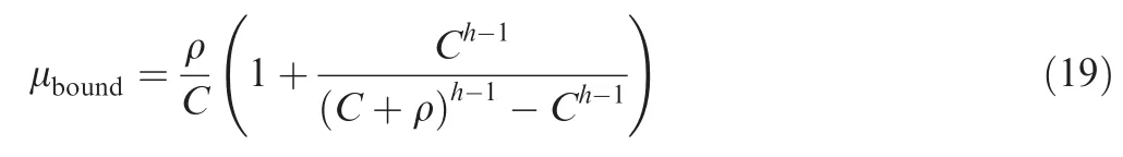
Here,the expression of μboundis still suitable for grouping strategy since fg(h)and f(h)have the same denominators.If the actual network utilization rate is higher than the corresponding μbound,the whole network may have no such an ability to schedule and forward all flows properly.Considering the fact that the constant bit rate of a single flow(or the average flow rate in an output port)usually is by far less than network link speed,a more simple expression for our basic end-to-end delay bound can be obtained by using(Ch+hρCh-1)to replace(C+ρ)h.

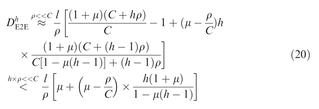
Thus,the maximal reachable boundary for the simplified delay bound iswhich also coincides with the basic GR model.11According to this boundary,if the maximal hop is one or two,the deterministic delay bound can always be calculated out,which means that the possibly maximal network utilization rate could be 100%.If h≥3,the calculation depends on utilization rate μ,for example,if h=3,the boundary of μ is 50%;if h=4,the boundary is 33%.Generally speaking,the possibly maximal network utilization rate is recommended not to exceed the corresponding reachable boundary,otherwise the worst-case end-to-end delay might be incalculable.Since the typical maximum of flow hop for industrial switched networks is 4,the recommended network load should be limited to 33%according to our theory,which also coincides with the actual network utilization rate of 25%for A380-like AFDX with up to 4 hops for flows.A more accurate model for the maximal reachable boundary can beif the one-order term expression of ρ is considered in Eq.(19).

6.3.Grouping ability comparison

In Section 5,we have given the measurement for grouping ability.Since grouping strategy can tighten the end-to-end delay upper bound,it is quite meaningful to get to know at what degree grouping strategy could increase the bound tightness.First,the in fluence of parameters μ,ρ and h on grouping ability under a given network connecting degree(such as Deg=6)is investigated.The results are shown in Fig.7.

When Deg is assigned with different values,the in fluence caused by network connecting degree can be observed,and the results are shown in Fig.8.

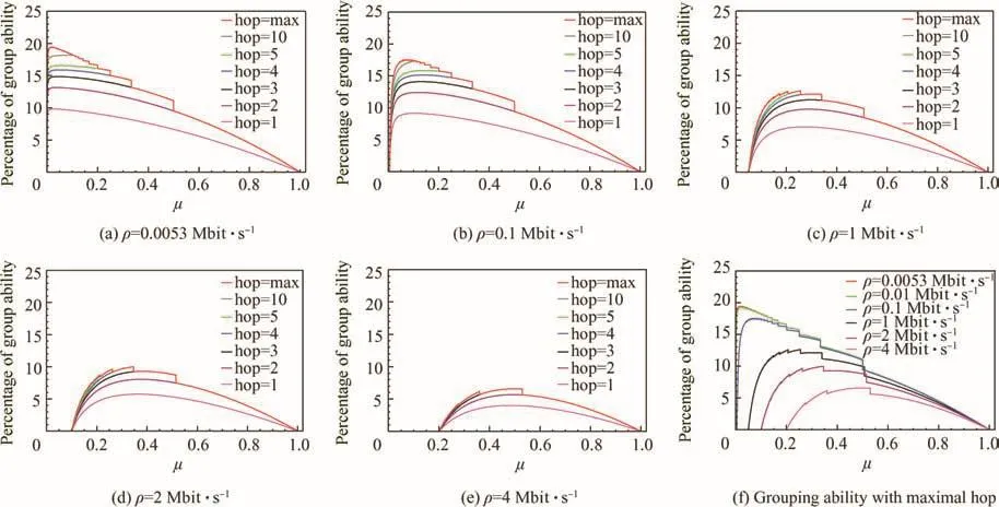
Fig.7 Grouping ability comparison under Deg=6.

With the increase of Deg,the corresponding possible grouping ability drops because the well-distributed assumption for flows just wipes out the advantage from grouping strategy when Deg is assigned to a relatively big value.Also,we can find that grouping ability increases quickly when μ gets a little increase from the starting point,and this trend just theoretically provides a good infrastructure for the adoption of grouping strategy to tighten the end-to-end delay bound.

6.4.Comparison with complete network calculus method

In this section,a further discussion about the comparisons between our deterministic upper bounds and the complete network calculus method will be performed.A fully connected topology is selected out for the comparisons,which is shown in Fig.9.This chosen topology includes 12 end systems and 4 switches.Each switch is connected with other 3 switches and 3 end systems with the link speeds as 100 Mbit·s-1.Thus,the network connecting degree in this topology is Deg=6 and the maximal flow hop is h=2 when all flows follow the shortest path routing algorithm.

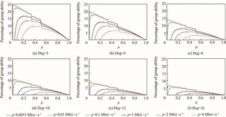
Fig.8 In fluence of networking degree on grouping ability.

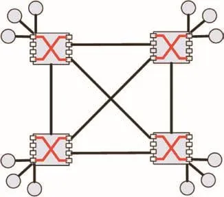
Fig.9 Fully connected network topology with h=2.

In order to make the comparison more general,all flows are randomly generated.Focused on a certain flow,its source and destination will be assigned randomly from a set of nodes.Typically,the flow constant rate will be generated according to two modes.For the uniform flow constant rate mode,every flow has the same rate ρ.Flow packet length Lmaxwill be selected out randomly from the range of[84,l]bytes.Here,l is the maximal permitted packet length designed by architecture designers.According to ρ and Lmax, flow period P(or the minimal interval)can be calculated out.For the average flow constant rate mode,there is not a uniform ρ for every flow.Each flow’s parameters will be assigned randomly from the range of[1,128]ms for period P and the range of[84,l]bytes for packet length Lmax.The average¯ρ will be calculated when flow generation is finished.No matter which generating mode is adopted,the utilization rate in each node will be checked to ensure the restriction by the upper bound μ.When all nodes are fully filled with flows,an auto path generating method will be used to compute each flow’s path according to the shortest path algorithm with load balance strategy.Finally,the bandwidth usage rate of each output port at every switch will be checked.If the actual usage is more than the designated μ,the actual value will be used to replace the original one.

When all flows have been generated and paths been planned,the complete network calculus method is implemented for the worst-case delay computing for each flow.Also the whole network is investigated to obtain the corresponding group capacity N for our deterministic upper bounds.The comparison results are shown in Table 1 and 2.The maximal values of BNC(Basic Network Calculus)and GNC(Grouping Network Calculus)come from the complete network calculus method,and the average group benefit is calculated from the statistic data for all flows according to BNC and GNC.The values of the maximal permitted packet length l originate in the scope of packet length in AFDX,in which the minimal packet length is 84 bytes and the maximal packet length is 1538 bytes both including the inter frame gaps(12 bytes)and preambles(1+7 bytes).

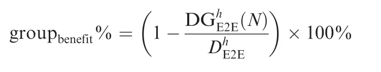
From Tables 1 and 2,we can find when all flows have the same packet length(l=84 bytes),our novel basic upper boundand grouping upper boundare very close to the actually maximal delays from the complete network calculus computing.Though the estimation accuracy of our upper bounds drops a little for the average flow constant rate case,the effectiveness of our upper bounds exceeds 80%.If packet lengthsvary considerably (such asfrom 84 to 1538 bytes),the effectiveness of our upper bounds shrinks to 40%,which means that the actual network calculus delays may be less than the half of our basic upper bound or grouping upper bound.Since the upper limit l of packet length in our model wipes out all of the detailed information about each flow’s packet length no matter what sizes it would be,the downward trend for the estimation effectiveness is reasonable for a big varying range of packet length.Besides,the assumption that all other aggregating flows have experienced their maximal hops during the analysis process of our bounds also increases the pessimism.What’s more,this kind of effectiveness of our deterministic bounds is based on the tremendous reduction about the switched networking parameters and computing amount.For example,our bounds only need six abstracted parameters about switched networking features:link speed C,bandwidth utilization rate μ, flow constant bit rate ρ,upper limit of packet length l, flow hop h and group capacity N.But the complete network calculus method needs every flow’s detailed parameters and information about networking topology.This kind of difference brings great advantage of our models for computing speed.Results in Tables 1 and 2 also show that the grouping benefit(groupbenefit%)of our bounds is quite close to the actually average group benefit which is acquired according to every flow’s BNC and GNC delays within the whole network.The grouping advantages from both the actual network calculus results and our deterministic grouping upper bound are around 18%–22%,9which also well match the statistic benefit as 24.2%in Ref.for an industrial AFDX network.

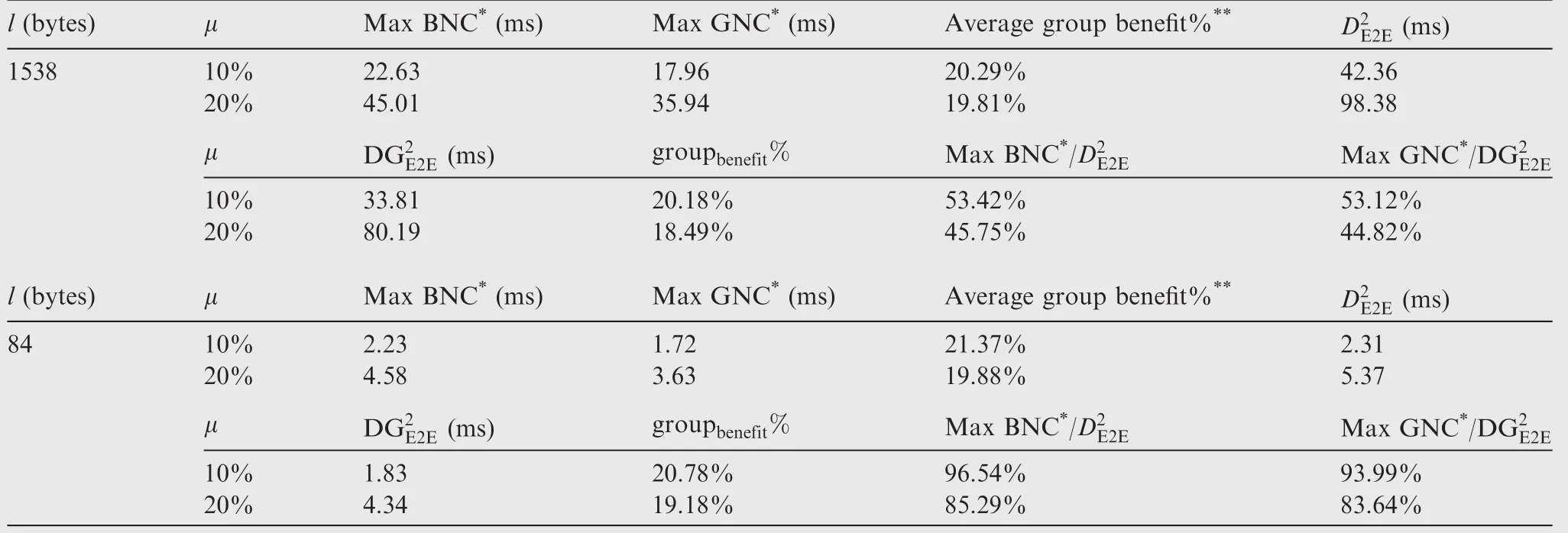
Table 1 Delay comparison for uniform flow constant rate case(ρ =0.1 Mbit·s-1).

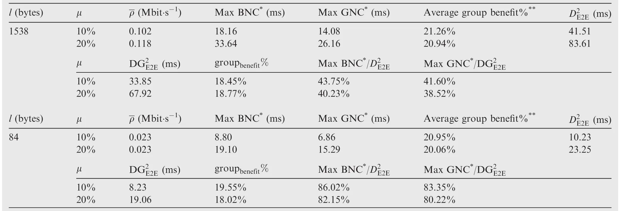
Table 2 Delay comparison for average flow constant rate case.

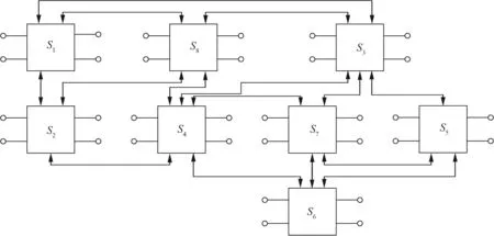
Fig.10 A typical AFDX network with maximal hop as 4.

6.5.Industrial case study

Focused on an industrial case,17we will show in which way our upper bounds can be used to predict the worst-case delay bound.The AFDX con figuration is composed of 8 switches with a maximal flow hop as 4 and maximal network connecting degree as 9.The link speeds of all physical connections are the same as 100 Mbit·s-1.There are more than 1000 Virtual Links transmitting and forwarding within the whole network.Bauer et al.7also mentioned this industrial case and showed that the total number of VLs was 1063.The topology of this case is shown in Fig.10.

Since the count of the access connections(32 access links)are more than the number of the backbone links(15 backbone links),the bandwidth utilizations of the backbone links should be higher than those of the access links.Thus,we pay more attention to the backbone links.Besides,no information is provided in Ref.17about the maximal packet length,and we assume that it obeys the basic restriction in AFDX.In the following analysis,the maximal permitted packet length is assigned as 1538 bytes.

According to our models,if the maximal bandwidth utilization among the backbone links is around 10%(or 20%),the basic upper bound and grouping upper bound are about 89.5 ms and 81.4 ms(or 318.6 ms and 289.6 ms for 20%utilization)respectively.The calculated upper bounds for 20%utilization case are quite bigger than those for 10%case and even scale out the scope of VL bandwidth allocation gaps(1–128 ms).3In fact,if the topology shown in Fig.10 can be modified with a better connecting ability to ensure that the maximal flow hop could be limited into 3,a much smaller bound can be guaranteed.In order to achieve this,two physical links should be added:one connects S1and S6,and another connects S2and S5.What’s more,the additional two lines do not increase the whole network connecting degree.According to this modified topology,the basic upper bounds and grouping upper bounds are 63.0 ms and 57.7 ms,171.9 ms and 157.5 ms for 10%and 20%utilizations respectively,which are improved remarkably from the original topology design.

In order to illustrate the effect of the maximal flow hop more clearly,two sets of VLs will be used to imitate the practical avionics con figurations:one set includes 1600 VLs and another set includes 3200 VLs.These VLs are randomly generated according to the uniform flow constant rate mode,which is consistent with the method discussed in Section 6.4.For the case containing 1600 VLs,the bandwidth utilization of each node among the 32 end systems is about 5%,which leads to a peak utilization among the backbone links up to 10.4%for the original topology and 7.3%for the modified topology.For the case containing 3200 VLs,the bandwidth utilization of each end system is about 10%,furthermore leading up to 20.2%utilization for the original topology and 13.8%for the modified topology among the backbone links.Since the modified topology has a better control for network connecting,the maximal bandwidth utilizations are obviously smaller than the original topology under the same access loads,as well as better deterministic bounds.The comparative results are shown in Table 3.Also we show BNC and GNC results according to the complete network calculus method for contrast.

Both the complete network calculus method and our deterministic upper bound analysis method show that the worstcase delays for the modified topology are obviously cut down from the original one since flow hops are restricted into 3 switches within the modified case.When the access load is 5%,the improvements for Max BNC and Max GNC methods according to the complete network calculus are 35.1%and 29.4%respectively,and the improvements for DE2Eand DGE2Emethods are 56.3%and 45.4%respectively.When the access load is 10%,the improvements are even more remarkable than those for 5%load case.The grouping advantages for the original topology from the complete network calculus results are still around 24%–25%,which are in close proximity to the benefit as 24.2%in Ref.9Our deterministic analysis methods also support this.For the modified case,the grouping advantages drop to 15%–16%because of a more even dispatch of link utilizations among the backbone switches.

From the analysis process for the AFDX industrial case,it just shows at what degree the maximal flow hop could affect the final end-to-end delays.Also,it illustrates how our deterministic upper bounds can be used to predict network performance and help to optimize the networking.

7.Conclusions

The main job of this paper can be divided into three parts:(A)carry on the research about the upper bound of end-to-end delays for switched networks;(B)investigate grouping benefit from grouping strategy and establish a measurable model for grouping ability;(C)compare the proposed upper bound with other analysis methods and illustrate its effectiveness in typical networking cases.The contributions of this paper can be summarized as follows:

(1)A novel method is proposed to estimate the deterministic upper bound of end-to-end delays for switched networks according to some typical networking features.Two deterministic upper bounds are obtained from network calculus prospective:the first one is for a basic switched networking condition,while the second one is based on the philosophy of grouping strategy.Not like using NC and TA methods to get each flow’s WC delay(during these calculus processes,the detailed con figurations are needed,such as Topology,routing paths,and VLs),the upper bounds in the paper are only based on some typically abstracted parameters.So the final bounds are for the whole network but not for each flow individually.These two upper bounds just give a general performance pro file for a switched network,especially in avionics context.According to the comparison results,our basic bound can achieve better performance than two typical GR bounds especially when the utilization rate of the whole network is no more than 50%.Even compared with the results from the complete network calculus method for a fully connected network with 4 switches and 12 end systems,the effectiveness of our bounds exceed 80%when flow packet lengths keep the same.If flow packet lengths vary considerably(such as from 84 to 1538 bytes),the effectiveness of our bounds is no less than 38%.

(2)Based on the concept of network connecting degree,a theoretical expression of the minimal grouping ability for a general switched network is established.The grouping ability of a whole switched network is about15%–20%if the average flow constant rate is limited within[0.0053,0.1]Mbit·s-1and the utilization rate of the switched network is no more than 30%.This theoretical result just coincides with the actual grouping advantage(18%–22%)when all flows are generated randomly within a fully connected topology with 4 switches and 12 end systems.Besides,the grouping advantage(24%–25%)from two sets of VLs containing 1600 and 3200 flows respectively within an industrial airplane networking case also supports the grouping ability analysis.All the three results well match the statistical data(24.2%)shown in Ref.9.

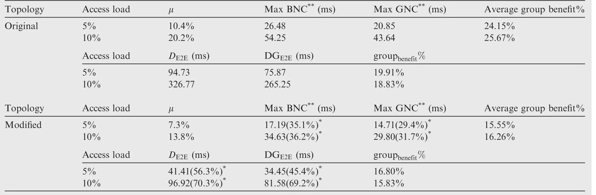
Table 3 Delay comparison for an industrial case(ρ =0.1 Mbit·s-1).

(3)According to the proposed upper bounds in this paper,the maximum reachable utilization boundary of a switched network is proposed,which can be used to restrict the networking utilization.For a typically switched network,like the AFDX network for A380,the maximal flow hop is limited to 4.Thus,the maximal networking utilization according to our model is recommended not to exceed 33%.And this theoretical result also coincides with the actual network utilization(about 20%–25%)for A380-like AFDX.

With the aid of our bounds,we can reconsider the design process from the overall perspective for a switched network.Traditionally,the analysis of the worst-case delay according to some analytic methods(such as network calculus and trajectory approach)is a post-veri fication method.With our deterministic upper bounds or some other methods,30the worstcase performance guarantee by design can be predetermined.Further studies are still needed in this direction.

Acknowledgements

This study was supported by the National Natural Science Foundation of China(No.61301086,71701020).

Appendix A.Network calculus with grouping strategy

A.1.Basic network calculus approach

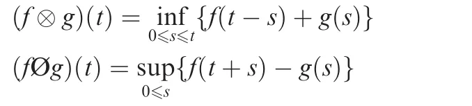
Network Calculus(NC)is a theoretical framework which provides deep insights into flow problems encountered in networking,especially for the problem of computing the end-to-end delays.NC is mathematically based on the Min-Plus dioid(also called Min-Plus algebra)13,for which the convolution⊗and deconvolution Ø operations between two functions f(t)and g(t)are de fined by

The basic concepts in NC are arrival curve and service curve.According to its theory,a flow R(t)has an arrival curve α(t)ifand a server has a service curve β(t)ifwhere R*(t)is the output flow for R(t).In this case,α*(t)=(αØβ)(t)is the arrival curve for R*(t)and can be used for the following aggregate behaviour.

The worst-case latency for flow R(t)when it is served by an output port with a service curve β(t)is the maximum horizontal difference between α(t)and β(t)and can be formally de fined by h(α，β)=sups≥0(inf｛τ≥ 0|α(s) ≤ β(s+ τ)｝).The end-to-end worst-case delay for flow R(t)is the sum of all latency in the corresponding output ports along its transmission paths.

If a flow strictly obeys the leaky bucket model,such as a VL in the AFDX network,its arrival curve can be simplified as ασ，ρ(t)= σ + ρt(t≥ 0),where σ is the maximal burst and ρ is the long-term bit rate.When flow’s period P and maximal packet length Lmaxare considered,these two parameters can be specified as Lmaxand ρ=Lmax/P.A typical example for the service curve is the rate-latency service curve with C as the service rate(such as 100 Mbit·s-1)and T as the maximal technology latency of the switch(such as 10 μs).Thus,it can be de fined as βC，T(t)=C[t-T]+.According to these models,the worst-case latency D can be easily calculated out and the uncertainty of flow’s arrival for the next aggregate nodes can be represented by a change of burstiness.Thus the arrival curve for R*(t)should be restricted by

A.2.Grouping strategy

It has been proved that the basic network calculus approach is quite pessimistic for the end-to-end performance evaluation.If grouping strategy is applied to the basic model,the average advantage is about 24.2%for an industrial AFDX network with nearly 1000 VLs.9The philosophy of grouping strategy lies in the fact that packets coming from the same node cannot be transmitted out at the same time by the output port.Consequently,the corresponding flows containing these packets can be seen as a group and the arrival curve for the group should be restricted by the speed of the physical link,which will lead to an in flection in the arrival curve.If there are several groups,the final arrival curve for all coming flows should be a concave increasing piecewise line with knowable piecewise slopes and in flection points.

1.Nam MY,Lee J,Park KJ,Sha L,Kang K.Guaranteeing the endto-end latency of an IMA system with an increasing workload.IEEE Trans Comput 2014;63(6):1460–72.

2.Nesrine B,Katia JR,Scharbarg JL,Fraboul C.End-to-end delay analysis in an Integrated Modular Avionics architecture.18th conference on emerging technologies and factory automation;2013 Sep 10–13;Cagliari,Italy.Piscataway(NJ):IEEE Press;2013.p.1–4.

3.ARINC 664 P7:ARINC speci fication 664.Aircraft data network,Parts 7:Avionics full-duplex switched ethernet network.Aeronautical Radio Inc.,Annapolis,MD;2005.

4.Boyer M,Fraboul C.Tightening end to end delay upper bound for AFDX network calculus with rate latency FIFO servers using network calculus.IEEE international workshop on factory communication systems;2008 May 21–23;Dresden,Germany.Piscataway(NJ):IEEE Press;2008.p.11–20.

5.Liu C,Wang T,Zhao CX,Xiong HG.Worst-case flow model of VL for worst-case delay analysis of AFDX.IET Electron Lett 2012;48(6):327–8.

6.Scharbarg JL,Ridouard F,Fraboul C.A probabilistic analysis of end-to-end delays on an AFDX avionic network.IEEE Trans Indust Inform 2009;5(1):38–49.

7.Bauer H,Scharbarg JL,Fraboul C.Improving the worst-case delay analysis of an AFDX network using an optimized trajectory approach.IEEE Trans Indust Inform 2010;6(4):521–33.

8.Bauer H,Scharbarg JL,Fraboul C.Applying trajectory approach with static priority queuing for improving the use of available AFDX resources.Real-Time Syst 2012;48:101–33.

9.Bauer H,Scharbarg JL,Fraboul C.Applying and optimizing trajectory approach for performance evaluation of AFDX avionics network.Proceeding of the 14th international conference on emerging technologies and factory automation;2009 Sep 22–25;Palma de Mallorca,Spain.Piscataway(NJ):IEEE Press;2009.p.1-–8.

10.Gutie´rrez JJ,Palencia JC,Harbour MG.Holistic schedulability analysis for multipacket messages in AFDX networks.Real-Time Syst 2014;50:230–69.

11.Le Boudec JY,Thiran P.Network calculus:a theory of deterministic queuing systems for the internet.Berlin,Germany:Springer;2001.p.67–75.

12.Duan ZH,Zhang ZL,Hou YT.Fundamental trade-offs in aggregate packet scheduling.IEEE Trans Parallel Distrib Syst 2006;16(12):1166–77.

13.Cruz RL.A calculus for network delay,part I,network elements in isolation.IEEE Trans Inf Theory 1991;37(1):114–31.

14.Adnan M,Scharbarg JL,Ermont J,Fraboul C.Model for worst case delay analysis of an AFDX network using timed automata.IEEE conference on emerging technologies and factory automation;2010 Sep 13–16;Bilbao,Spain.Piscataway(NJ):IEEE Press;2010.p.1–4.

15.Ermont J,Fraboul C.Modeling a spacewire architecture using timed automata to compute worst-case end-to-end delays.IEEE 18th conference on emerging technologies&factory automation;2013 Sep 10–13;Cagliari,Italy.Piscataway(NJ):IEEE Press;2013.p.1–4.

16.Grieu J.Analyse et valuation de techniques de com-mutation Ethernet pour l’interconnexion des systmes avioniques[dissertation].Toulouse:Laboratory Space and Aeronautical Telecommunications;2005.

17.Charara H,Scharbarg J,Ermont J,Fraboul C.Methods for bounding end-to-end delays on an AFDX network.IEEE 18th euromicro conference on real-time systems;2006 July 6–7;Dresden,Germany.Piscataway(NJ):IEEE Press;2006.p.193–202.

18.Frances F,Fraboul C,Grieu J.Using network calculus to optimize the AFDX network.Proceedings of ERTS;2006.p.1–8.

19.Bouillard A,Nowak T.Fast symbolic computation of the worstcase delay in tandem networks and applications.Perform Eval 2015;91:270–85.

20.Zhao LX,Pop P,Li Q,Chen JY,Xiong HG.Timing analysis of rate-constrained traf fic in TTEthernet using network calculus.Real-Time Syst 2017;53(2):254–87.

21.De Azua Ruiz JA,Boyer M.Complete modeling of AVB in network calculus framework.Proceeding of 22nd international conference on real-time networks and systems;2014.p.55–64.

22.He F,Zhao L,Li ES.Impact analysis of flow shaping in ethernet-AVB/TSN and AFDX from network calculus and simulation perspective.Sensors 2017;5(17):1181–214.

23.Li XT,Cros O,George L.The trajectory approach for AFDX FIFO networks revisited and corrected.Proceeding of the 2014 IEEE 20th international conference on embedded and real-time computing systems and applications;2014 Aug 20–22;Chongqing,China.Piscataway(NJ):IEEE Press;2014.p.1–10.

24.Li XT,Scharbarg JL,Fraboul C.Analysis of the pessimism of the Trajectory approach for upper bounding end-to-end delay of sporadic flows sharing a switched Ethernet network.Proceeding of 19th international conference on real-time and network systems;2011.p.149–58.

25.Li XT,George L.Deterministic delay analysis of AVB switched Ethernet networks using an extended trajectory approach.Real-Time Syst 2017;53(1):121–86.

26.Suthaputchakun C,Sun ZL,Kavadias C,Ricco P.Performance analysis of AFDX switch for space onboard data networks.IEEE Trans Aerosp Electron Syst 2016;52(4):1714–27.

27.Ashjaei M,Behnam M,Nolte T.SEtSim:a modular simulation tool for switched Ethernet networks.J Syst Architect 2016;65:1–14.

28.Kemayo G,Benammar N,Ridouard F,Bauer H,Richard P.Improving AFDX end-to-end delays analysis.Proceeding of IEEE 20th conference on emerging technologies&factory automation(ETFA);2015 Sep 8–11;Luxembourg,Luxembourg.Piscataway(NJ):IEEE Press;2015.p.1–8.

29.Li J,Yao JY,Huang DS.Ethernet-based avionic databus and time-space partition switch design.J Commun Networks 2015;17(3):286–95.

30.Kang K,Nam MY,Sha L.Worst case analysis of packet delay in avionics systems for environment monitoring.IEEE Syst J 2015;9(4):1354–62.

9 December 2016;revised 6 March 2017;accepted 8 June 2017

Available online 9 September 2017

Ⓒ2017 Chinese Society of Aeronautics and Astronautics.Production and hosting by Elsevier Ltd.This is an open access article under the CCBY-NC-ND license(http://creativecommons.org/licenses/by-nc-nd/4.0/).

*Corresponding author.

E-mail address:robinleo@buaa.edu.cn(F.HE).

Peer review under responsibility of Editorial Committee of CJA.