Yun Long (龙云), Xin-ping Long (龙新平), Bin Ji (季斌), Wen-xin Huai (槐文信), Zhong-dong Qian (钱忠东)

1.State Key Laboratory of Water Resources and Hydropower Engineering Science, Wuhan University, Wuhan 430072 China

2.HubeiKey Laboratory of Waterjet Theory and New Technology, School of Power and Mechanical Engineering, Wuhan University, Wuhan 430072, China

3.Science and Technology on Water Jet Propulsion Laboratory, Shanghai 200011, China, E-mail: whulongyun@whu.edu.cn

Verification and validation of URANS simulations of the turbulent cavitating flow around the hydrofoil*

Yun Long (龙云)1,2,3, Xin-ping Long (龙新平)1,2, Bin Ji (季斌)1,2,3, Wen-xin Huai (槐文信)1, Zhong-dong Qian (钱忠东)1

1.State Key Laboratory of Water Resources and Hydropower Engineering Science, Wuhan University, Wuhan 430072 China

2.HubeiKey Laboratory of Waterjet Theory and New Technology, School of Power and Mechanical Engineering, Wuhan University, Wuhan 430072, China

3.Science and Technology on Water Jet Propulsion Laboratory, Shanghai 200011, China, E-mail: whulongyun@whu.edu.cn

In this paper, we investigate the verification and validation (V&V) procedures for the URANS simulations of the turbulent cavitating flow around a Clark-Y hydrofoil. The main focus is on the feasibility of various Richardson extrapolation-based uncertainty estimators in the cavitating flow simulation. The unsteady cavitating flow is simulated by a density corrected model (DCM) coupled with the Zwart cavitation model. The estimated uncertainty is used to evaluate the applicability of various uncertainty estimation methods for the cavitating flow simulation. It is shown that the preferred uncertainty estimators include the modified Factor of Safety (FS1), the Factor of Safety (FS) and the Grid Convergence Index (GCI). The distribution of the area without achieving the validation at theUvlevel shows a strong relationship with the cavitation. Further analysis indicates that the predicted velocity distributions, the transient cavitation patterns and the effects of the vortex stretching are highly influenced by the mesh resolution.

Cavitating flow, cavitation, verification and validation (V&V), uncertainty

Introduction

In the past, much attention was paid on the cavitating flow for its complicated two-phase flow features[1-3]. Numerous experimental and numerical researches were conducted and many significant phenomena and mechanisms were revealed[4-6]. The cavitation can be divided into four stages, the incipient stage, the sheet stage, the cloud stage and the super cavitation stage[7]. The nuclei size and the nuclei density were considered by Arndt as the main factors for the cavitation inception[8], and related researches[4]were conducted for understanding the mechanism of the cavitation inception. Violently unsteady and quasiperiodic process is observed due to the sheet/cloud cavitation shedding. The re-entrant jets were claimed to be responsible for the cloud cavitation shedding based on the experimental and numerical investigations[9-11]. More recently, Peng et al.[12]observed the U-type flow structures around the hydrofoils in the cavitation tunnel. It is a common phenomenon in the U-type flow structures with the cloud cavity. All these show the great complexity and difficulties in the cavitation research. So far, there have been no unified explanations and conclusions for the cavitation.

It is worth mentioning that the numerical simulations have achieved a remarkable progress for the cavitating flow in the last two decades[1]. The Reynolds-averaged Navier-Stokes (RANS) simulations were widely applied in the cavitation flow andpractical applications[13-16]. Numerical methods such as the large eddy simulation (LES)[17-20]are more accurate than the RANS and are widely used nowadays in the cavitating flow simulations. However, little attention has been paid on the verification and validation (V&V) in the cavitating flow simulations with the RANS or LES methods, although it was well understood that the mesh in fluence was a great concern[3,11,16]. The V&V is a basic procedure to evaluate the reliability before accepting the simulated results. In our previous study[18], it was suggested that the V&V is an important and essential part of the CFD. In view of the violently unsteady flow feature and the high noise level, the numerical results may contain a great number of uncertainties and variations in the cavitation simulations. Thus, the V&V of the cavitating flow simulations should be an urgent issue to be investigated and applied in the practice.

The current quantitative uncertainty estimates for the RANS are mainly built based on the Richardson extrapolation methods. The Grid Convergence Index (GCI) proposed by Roache[21]is used extensively and recommended by American Society of Mechanical Engineers and American Institute of Aeronautics and Astronautics. The GCI and the variations of the grid convergence index, i.e., the Grid Convergence Index modified by Oberkampf and Roy (GCI-OR)[22], the grid convergence index modified by Logan and Nitta (GCI-LN)[23], and the Grid Convergence Index modified by Roache (GCI-R)[24], see a wide applications in many fields[21-25]. In the Correction Factor Method (CF) developed by Stern et al.[26], a correction factor is used to indicate how far away from the asymptotic range. Wilson et al.[27]expressed the assessments and put forward some modified ideas, and then the modified CF is recommended by the ITTC for the uncertainty analysis in the CFD V&V.

As pointed out by Xing and Stern[28]and Stern et al.[29], the GCI and the CF have two main drawbacks. The first drawback is that the estimated uncertainty is unreasonably small when the observed order of accuracy is less than the formal order of accuracy. The second drawback is that the confidence levels with few statistical evidence for the GCI and the CF are not well explored. In this context, the Factor of Safety Method (FS) and its modified version (FS1) were proposed by Xing and Stern[28,30]to overcome the two main drawbacks in the CF and the GCI. The FS and FS1 methods show the best conservativeness compared to other methods with large calculations in Xing and Stern’ s studies[28,30].

All these seven methods were evaluated with large amount of practice[21-28]. Most of these studies focus on the uncertainty estimation with much mitigating flow compared to the unsteady cavitating flow, but the calculation of solution quantities is at a high noise level in unsteady cavitating. Therefore, the appropriateness of all uncertainty estimators applied in the URANS simulations of the cavitating flow remains an issue for more studies and practices.

The current CFD V&V for the LES was proposed and applied[31-33], but with many unsolved problems even in the simulation of simple flow phenomena such as the channel flow. So far, there is no clear and practical guideline for the V&V of the LES applied in the engineering field. It is a challenging work for the V&V of LES in the future.

Inspired by the above studies, this paper pays attention to the V&V procedures for the URANS simulations of the turbulent cavitating flow around a Clark-Y hydrofoil. The main focus of this study is to investigate the feasibility of various Richardson extrapolation-based uncertainty estimators in the cavitating flow simulation. It is an attempt to carry on the V&V of URANS simulations of the turbulent cavitating flow, and also a preparation for future in-depth investigations of the LES V&V in the cavitation simulation. The experimental data in published papers[7,16]are chosen to carry on the validation procedure. Simulated cavitation results are discussed with respect to different mesh resolutions.

1. Numerical methods and uncertainty estimators

To simulate the unsteady cavitating flow, the standard RNGk-εturbulence model modified by the density corrected model (DCM)[34,35], whose advantages and accuracy in the cavitation simulation were widely validated[34-37], is employed coupled with a mass transfer cavitation model. The main features of the models are as follows.

1.1 Physical cavitation model

The Zwart model[38]is used to describe the mass transfer in the ANSYS CFX solver, and it was used and validated widely to accurately capture the feature of the cavitation. The mass transfer equation is as follows

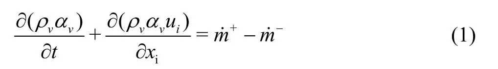
whereαvis the vapor volume fraction. The source termsandin Eq.(1) are the mass transfer rates for the vaporization and condensation processes, respectively. The Rayleigh-Plesset equation describing the single bubble dynamics is simplified as:

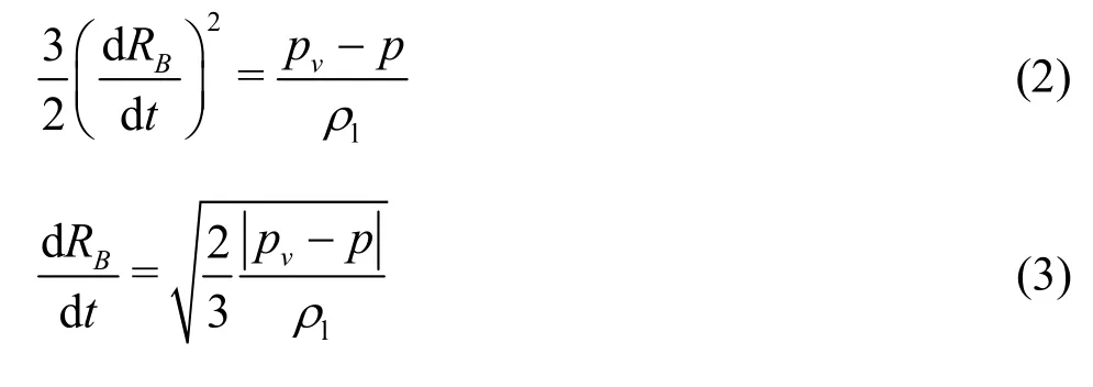
whereRBis the bubble diameter,pvis the saturated vapor pressure, andpis the local liquid pressure. The rate of change of the bubblemBcan be calculated as

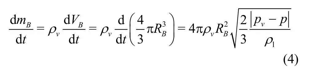
whereρvis the vapor density andVBis the bubble volume. If there areNBbubbles per unit volume, the volume fractionαvmay be expressed as

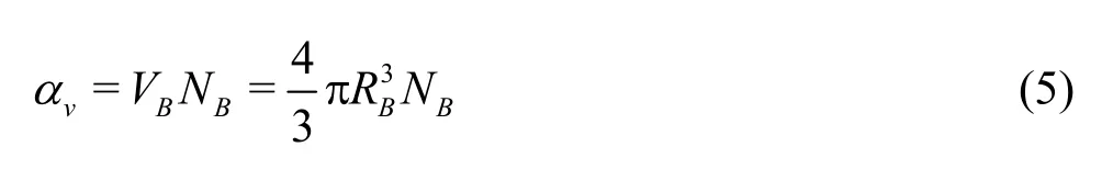
The total interphase mass transfer rate per unit volume is

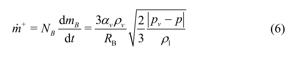
This expression is derived by assuming the vaporization. It can be generalized to include the condensation as

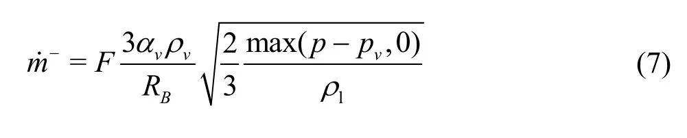
whereFis an empirical constant.Ftakes different values for the condensation and the vaporization in view of the fact that the condensation is usually much slower than the vaporization. The vaporization is initiated at the nucleation sites as usually the non-condensible gases. As the vapor volume fraction increases, the nucleation site density decreases. For the vaporization,αvis replaced byαnuc(1-αv)

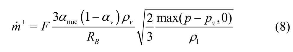
whereαnucis the volume fraction of the nucleation site. The model parameters are set as follows,for the

vaporization andFcond=0.01 for the condensation.

1.2 Density corrected model (DCM)

The standard RNGk-εmodel is based on the renormalization group analysis of the Navier-Stokes equations. To take into account the influence of the compressibility, which has a remarkable effect on the cavitating flow simulation, the standard RNGk-εmodel is modified by the DCM model in this study.

Coutier-Delgosha et al.[35]proposed a density corrected model (DCM), in which the turbulent eddy viscosityμTis modified as

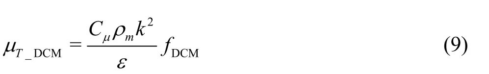
where the empirical constantCμis 0.09,kis the turbulent kinetic energy,εis the turbulent eddy dissipation,ρmis the mixture density, which is defined as

whereρlis the liquid density andαlis the local liquid volume fraction. The functionfDCMis expressed as

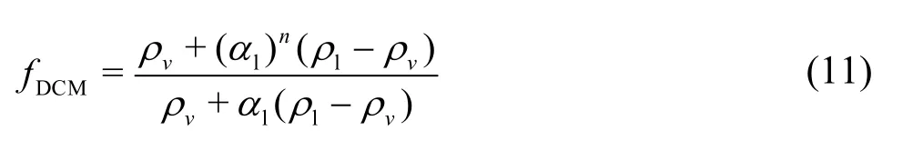
In this study, the constantnis set as 10[36,37].

1.3 Numerical setup

The unsteady cavitating flow around a Clark-Y hydrofoil is simulated by the DCM model coupled with a homogeneous cavitation model. The CFX Expression Language in the ANSYS CFX is used to implement the DCM model, and the scalable wall function is adopted.

The Clark-Y hydrofoil with a chord lengthC=0.07 m is placed horizontally in the computational domain at a fixed angle of attack ofα=8oas shown in Fig.1. The spanwise length is 0.3C. The adopted length and height in the computational domain are shown in Fig.1. The boundary velocity inlet is set asU∞=10 m/s, and the boundary outlet is imposed as a fixed static pressurepout=43079 Pa , which is derived by the cavitation numberσ=0.8No-slip boundary is applied on the hydrofoil surface. The upper and lower walls are arranged as free slip walls. The side wall boundary is arranged as the periodicity interface. An O-H type grid is used to generate the structural mesh for five sets of meshes. Five systematically refined meshes are used with a constant refinement ratioand The mesh 3 is shown in Fig.2. The detailed information about the five meshes is presented in Table 1.

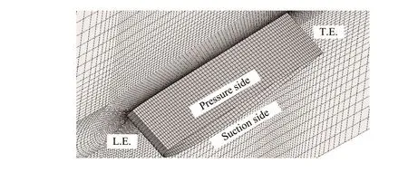
Fig.2 Structural mesh around the hydrofoil surface for mesh 3

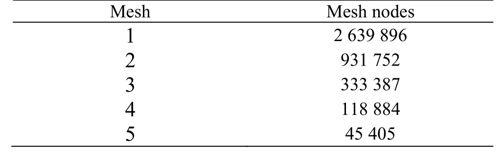
Table 1 Information about the five meshes

The time-dependent governing equations are discretized in both space and time domains. With consideration of the computational time and convergence, 20 iterations per time-step with 10-4residual criterion are used to achieve the balance of the accuracy and the efficiency. The uncertainty resulted by the residual criterion can be ignored compared to the grid. The time step is fixed as 10-4s as in Ref.[16] to investigate the influence of the grid. The higher order scheme is adopted for the convection terms with the second order backward Euler algorithm for the time integration. The simulations are carried out initially under the steady non-cavitation condition. Then, the unsteady cavitating flow is modeled with the steady cavitation results as the initial conditions. The convergence process is smooth and the results are displayed as follows.

1.4 Uncertainty estimators

The current uncertainty estimators are developed based on the Richardson Extrapolation Method. This paper focuses on the discretization uncertainty estimation with truncated power series expansions. The theoretical discretization errorδREis assumed as

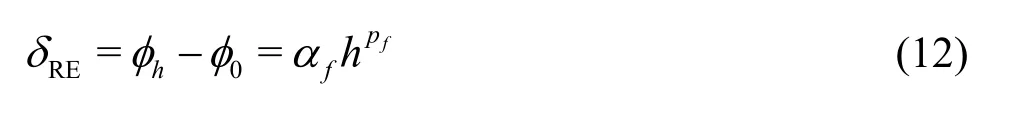
whereφhdenotes the solution with the grid spacingh,φ0stands for the exact solution of the discrete equations,αfis a constant, andpfis the formal order of accuracy.

The Richardson Extrapolation Method is derived from Eq.(12). The discretization error is estimated in the fine grid against three grids, i.e., the coarse grid Δx3, the medium grid Δx2, and the fine grid Δx1. Then, the fundamental elements to be used to estimate the uncertainty are as follows.

The constant grid refinement ratio is computed as

If the solutions for the coarse grid, the medium grid, and the fine grid areφ3,φ2andφ1,respectively, the change of the solutionεand the observed order of accuracypkcan be defined as:

The basic estimated error by the formal order of accuracypfor the observed order of accuracypk, as adopted in the seven estimators, can be defined as

The convergence ratioR[26]is expressed as

Then, the types of convergence can divide into four categories[39].

(1) Monotonic convergence: 0＜R＜1.

(2) Monotonic divergence: 1＜R.

(3) Oscillatory convergence: -1＜R＜0.

(4) Oscillatory divergence:R＜-1.

Based on the Richardson Extrapolation Method,if the solutions are asymptotic, and then the estimated uncertainty is the most accurate. As for the convergence ratioR, the monotonic convergence is required to obtain the uncertainty for the seven estimators (CF, FS, FS1, GCI, GCI-OR, GCI-LN, GCI-R). However, as Phillips and Roy[25]pointed out that it was very difficult and impractical to reach the rigorous conditions in practical applications, where very high noisy level is involved. Thus, all the estimators are modified by adding a minimum value 0.5 for the observed order of accuracy when the convergence is of the oscillatory type. This setup is an acceptable choice when solutions contain a high noise level in practical applications[25]. Obviously, with the monotonic divergence type, one can not determine the estimated uncertainty. Detailed descriptions of the discretization uncertainty estimations by the seven estimators discussed in this paper are as follows:

(1) Correction factor method (CF)

The CF developed by Stern et al.[26]and modified by Wilson et al.[27]is defined as

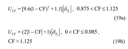
where

This correction factor is an indicator to show how far away from the asymptotic range.

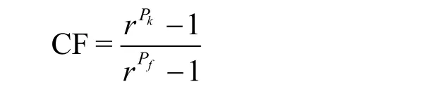
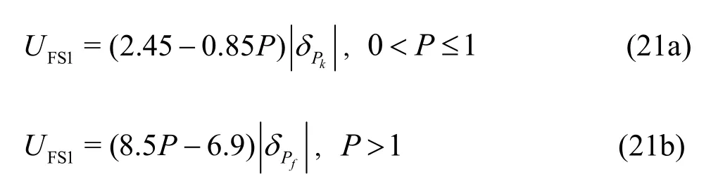
(2) factor of safety method (FS) and its modified version (FS1)

The FS developed by Xing and Stern[28]is defined as

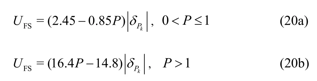
The FS1 is the modification proposed by Xing and Stern[30], which is defined as

(3) GCI and its modified versions (GCI-OR, GCI-LN, GCI-R)

The GCI developed by Roache[21]is defined as

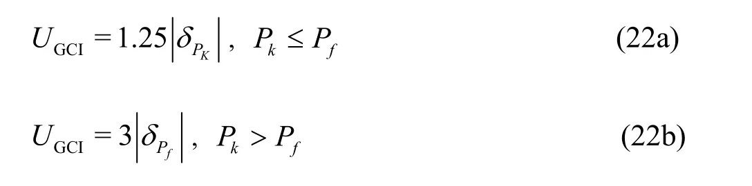
The modified version GCI-OR proposed by Oberkampf and Roy[22]is defined as

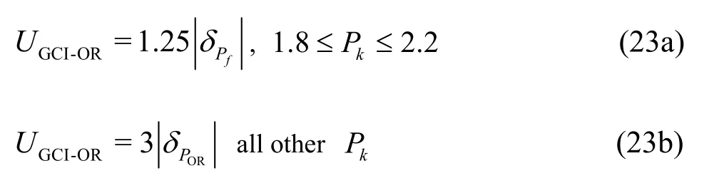
where

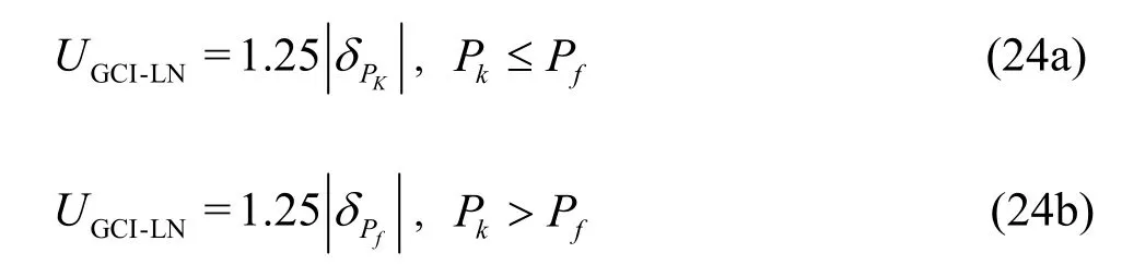
The modified version GCI-LN proposed by Logan and Nitta[23]is defined as

The GCI-R, a modification proposed by Roache[24], is defined as

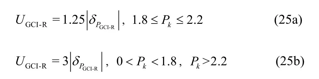
where

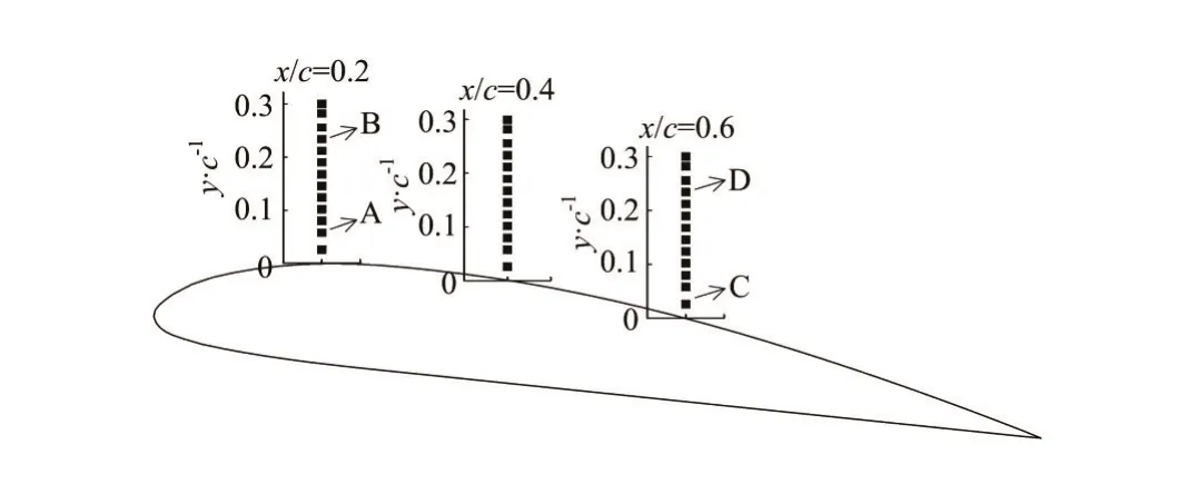
Fig.3 Monitoring points at selected chordwise locations along the foil

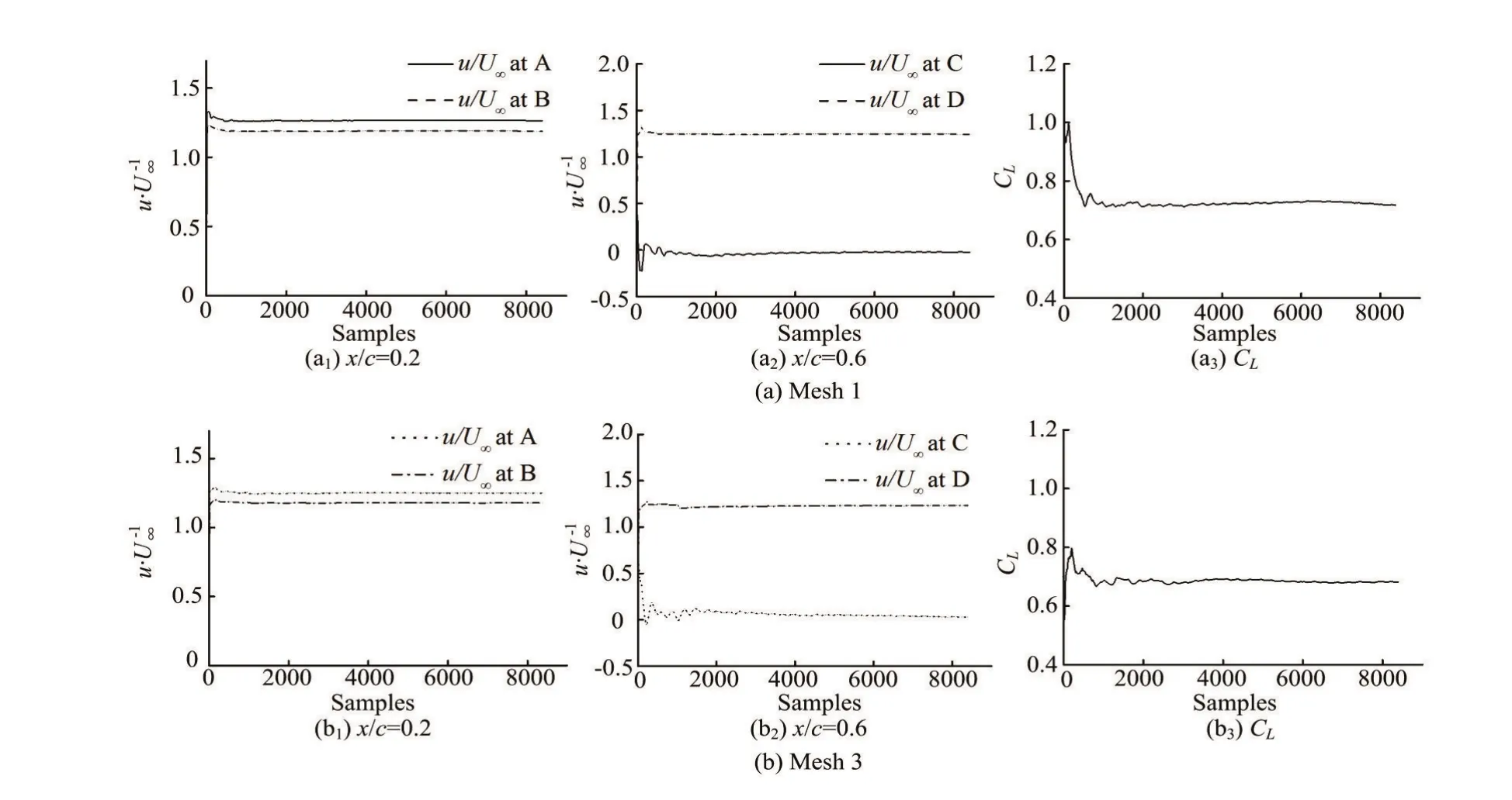
Fig.4 Moving average of the lift coefficient and normalized streamwise velocity at selected points along the foil forσ=0.8,α= 8o,

The CF and the GCI with various variations were widely used[21-27,40], but with two main drawbacks as pointed out by Xing and Stern[28,29]. The FS and the FS1 proposed by Xing and Stern are to overcome the two drawbacks, and they give a better uncertainty estimation in practical applications[25,28,30]. However, as mentioned before, the applicability and the feasibility of all these methods remain an issue to be explored for unsteady cavitating flows. The results of the studies and detailed discussions are as follows.

2. Results and discussions

2.1 Statistic convergence analysis

The monitoring points at the selected chordwise locationsx/c=0.2, 0.4 and 0.6 along the hydrofoil are shown in Fig.3. The points A, B, C, D are arranged as the representatives to investigate the statistic convergence. Figure 4 shows the evolution of the averaged values of different samples for the lift coefficientwhereCis the chord length,Sis the spanwise length) and the normalized streamwise velocityu/U∞at the selected points A, B, C, and D for mesh 1 and mesh 3, whereuis the predicted value at the monitoring location in the computational domain andU∞is the inlet velocity. From the results in Fig.4, at the beginning of the samples, the samples see a great influence on the averaged values, but it is clearly shown that the variations ofCLandu/U∞are relatively small at the end of samples. It can be said that the variation of the averaged value resulted from samples in this study has almost no effect on the estimated uncertainty.

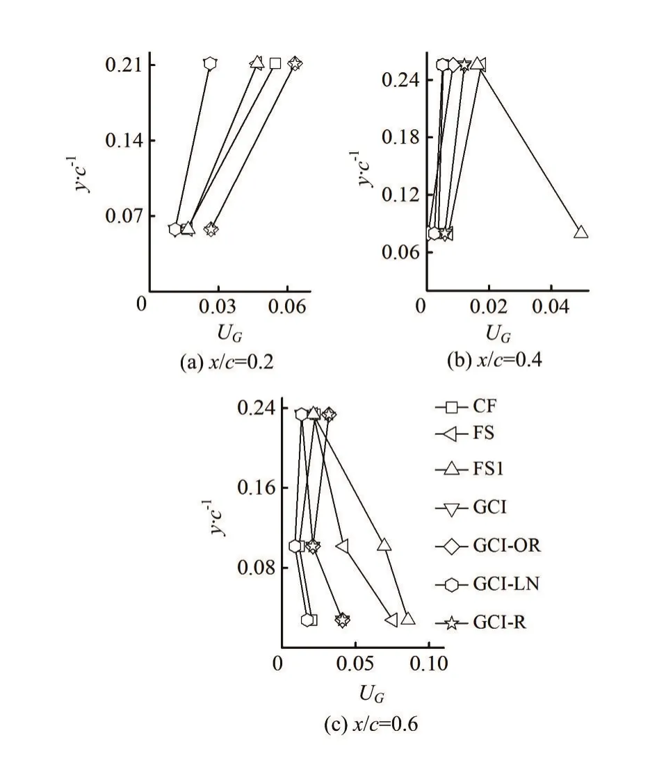
Fig.5 Distribution of discretization uncertainty at three chordwise locations for seven estimators

2.2 Discretization uncertainty estimation in unsteady cavitation flow

The discretization uncertainty UGfor the predicted value of the normalized averaged streamwise velocityu/U∞is obtained for seven estimators. Thepredictedu/U∞data are for the selected chordwise locationsx/c=0.2, 0.4 and 0.6.

The distribution of the estimated uncertainty at the three chordwise locations for seven estimators is presented in Fig.5. As shown in Fig.5, two locations at the vertical directiony/care selected atx/c=0.2 andx/c=0.4, representing the area near the foil and the area far away from the foil surface, respectively. Three locations at the vertical directiony/care selected atx/c=0.6, representing the area near the foil, the area of cavitation, and the area far away from the foil, respectively.

From Fig.5, it can be observed that the estimated uncertainty increases with the increase of the distance of the monitoring location from the foil surface for all estimators atx/c=0.2. However, atx/c=0.4, the estimated uncertainty by the FS1 becomes smaller with the increase of the distance of the monitoring location from the foil. This also happens atfor the FS1, the FS and the GCI. At, when the cavitation occurs, the estimated uncertainty for the CF, the GCI-OR, the GCI-LN and the GCI-R are the smallest as compared to other two vertical locations.

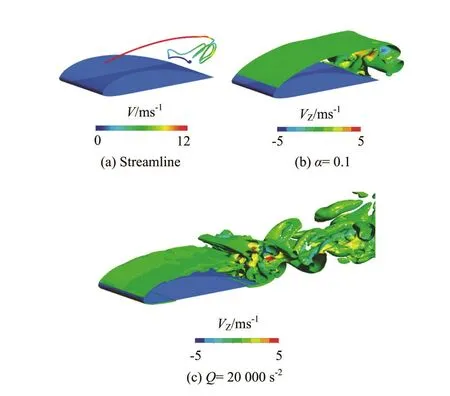
Fig.6 (Color online) Three-dimensional view of streamline and cavitation visualized by iso-surface of vapor volume fractionα=0.1 and vortex structures visualized by iso-surface ofQ-criterion[11],Q=20 000 s-2.σ=0.8,α= 8oand

For the cavitation flow, especially, for the highly unsteady cloud cavitation in this paper, as shown in Fig.6 and Fig.7, the velocity of the cavitation flow fluctuates violently due to the periodic shedding cavity[6,11,18]. The periodic shedding cavity can make the the solution quantities converge in a high noise level. Therefore, it is shown that the higher uncertainty appears in the area of cavitation and near the foil surface.

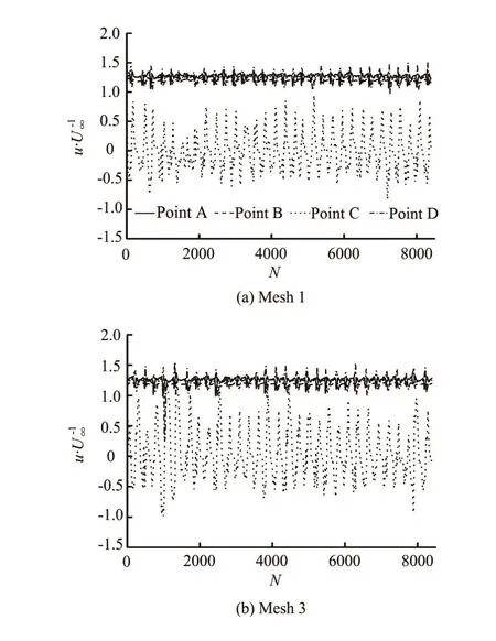
Fig.7 Fluctuation of normalized streamwise velocity at selected monitoring points along the foil.σ=0.8,α=8oandU∞=10 m/s

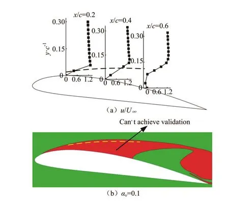
Fig.8 (Color online) The area without achieving validation at thelevel, distribution of experimentaland cavitation along the Clark-Y hydrofoil forσ=0.8,α=8oand

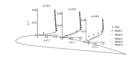
Fig.9 Comparisons of the experimental[16]and predicted normalized averaged streamwise velocities along the Clark-Y hydrofoil forσ=0.8,α=8oandU∞=10 m/s

In view of these observations, it may be concluded that the FS1, the FS and the GCI show better feasibility and applicability in the unsteady cavitation flow, and the FS1 may be the best choice to evaluate the uncertainty for the numerical simulation of the unsteady cavitating flow. All seven methods are mainly developed for the steady and no cavitation flow, but the unsteady cloud cavitation is a highly fluctuant two-phase flow. So their applications for the unsteady cavitation require more studies and practices in the future.

2.3 Discussion of the relationship between the cavitation and the uncertainty estimates

Figure 8 shows the comparison of the area without achieving the validation at theUvlevel and the distribution of the cavitation along the Clark-Y hydrofoil. When, it is said that the validation is achieved at theUvlevel[26]. The estimated uncertaintyUvis computed aswhereUSNis the numerical uncertainty, which is approximately equal to the discretization uncertaintyUGin this paper, andUDis the uncertainty of the experimental data[16]. In view of the high difficulty and uncertainty in measuring the data in the cavitating flow,UDis computed for 5% of the experimental results. Thedata indicated by the cubes in Fig.8(a) are the experimental results[16]for the selected chordwise locationsx/c=0.2, 0.4, 0.6. The area between the dotted line and the foil suction surface in Fig.8(a) is the area without achieving the validation at theUvlevel. The same area can be observed in Fig.8(b) between the dotted line and the foil suction surface. The red area in Fig.8(b) is predicted as the cavitation area, which is chosen as the representative from simulated transient cavitation results. The interface between the red and green areas is the iso-surface of the vapor volume fractionαv=0.1.

From Fig.8, it can be found that the area without achieving the validation at theUvlevel is located at where the cavitation occurs. The area without achieving the validation at theUvlevel shows a strong relationship with the cavitation, and the cavitation leads to a higher degree of difficulty to achieve the validation at theUvlevel. It is worth noting that the area without achieving the validation at theUvlevel is at the same locations whereUvis much less thanin this study (not shown here). It can be said that the modeling assumptions in this study need to be improved to capture the feature of the cavitation more accurately.

2.4 Evaluation of mesh resolution and cavitation simulation

Figure 9 presents the experimental[16]and predicted normalized averaged streamwise velocitiesat the selected monitoring locations along the Clark-Y hydrofoil. As shown in Fig.9, the predicted velocity distributions are in better agreement with the experimental results when the mesh resolution improves. It is a noticeable thing that there is a considerable deviation between simulated and experimental results in the cavitation area even with a fine mesh resolution.

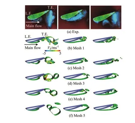
Fig.10 (Color online) Time evolution of cavitation shedding (experimental results are obtained from Ref.[16]. Simulated cavitation patterns are made by iso-surface of vapor volume fractionαv=0.1,σ=0.8 andU∞=10 m/s )

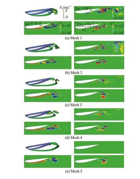
Fig.11 (Color online) Predicted vapor volume fraction, vortex stretching, vortex dilatation and baroclinic torque for five meshes.and10 m/s

Numerical snapshots for five meshes in Fig.10 are given to show the time evolution of the unsteady cavitation. The experimental results are from Ref.[16]. The experimental and numerical results from the left pattern to the right pattern denote that the unsteady cavity develops from the foil leading edge (L.E.), grows to its maximum at the trailing edge (T.E.), and sheds on the foil surface, respectively. From the picture, it can be observed that with the mesh resolution improving from the coarsest to the finest, the cavitation patterns become more complicated, and they are in better agreement with the experimental patterns. Note that the cavitation patterns predicted by the meshes 1, 2 and 3 have clearly demonstrated that the shedding cloud cavity turns from a two-dimensional cavity into a three-dimensional structure, but only two-dimensional cavity flows are observed by the meshes 4, and 5. This reveals that only when the mesh resolution reaches a certain high degree can the predicted cavitation results reflect the effect of the vortex stretching in the unsteady cloud cavitation, which represents the stretching and the tilting of the vortex due to the velocity gradients[11].

As shown in Fig.6 and Fig.10, the highly unsteady cavitating flow has a strong relationship with the complicated vortex structures. Thus, the vorticity transport equation is used to reveal the interaction between the cavitation and the vortex. It is used to investigate the influence of the mesh resolution on the vortex here. The vorticity transport equation in a variable density flow is employed as follows

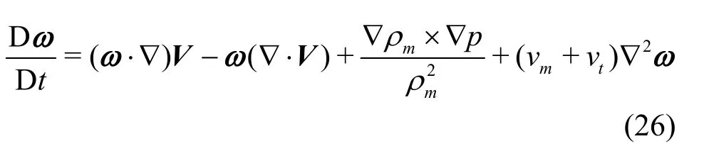
In this equation, the vorticity consists of three terms. The vortex stretching term (ω·∇)Vreveals the stretching and the tilting of a vortex due to the velocity gradients， the vortex dilatation termω（∇·V) is influenced by the volumetric expansion/contraction，and the baroclinic torquerepresents the generation of the vorticity for misaligned pressure and density gradients. The last term on the right side means the viscous diffusion of the vorticity, and it can usually be neglected in a high Reynolds number flow[11].

Figure 11 shows the predicted vapor volume fraction, the vortex stretching, the vortex dilatation and the baroclinic torque for five meshes when the unsteady cavity grows to its maximum at the trailing edge. From Fig.11, it can be seen that the mass transfer along the cavity surface has a significant effect on the vortex dilatation and the baroclinic torque. The baroclinic torque is mainly on the liquidvapor interface. This is in accordance with our previous studies[6,11]. When the mesh resolution decreases, the effect of the vortex becomes weaker in the flow field. It is worth noting that the effect of the vortex stretching becomes weaker and weaker, and it almost disappears especially for the mesh 5. This demonstrates again that only when the mesh resolution reaches a certain high degree can the predicted results reflect the effect of the vortex stretching in the unsteady cloud cavitation.

3. Conclusions

The unsteady cavitating flow around a Clark-Y hydrofoil is simulated by the DCM model coupled with the Zwart cavitation model and the results are analyzed by uncertainty estimate methods. The main conclusions are as follows:

(1) The FS1, the FS and the GCI show better feasibility and applicability in the unsteady cavitation flow, and the FS1 may be the best choices for evaluating the uncertainty.

(2) The area without achieving the validation at theUvlevel shows a strong relationship with the cavitation and the cavitation can lead to a higher degree of difficulty to achieve the validation at thelevel.

(3) When the mesh resolution improves, the predicted velocity distributions and the cavitation patterns are in better agreement with the experimental results. Moreover, only when the mesh resolution reaches a certain high degree can the predicted cavitation results reflect the effects of the vortex stretching in the unsteady cloud cavitation.

It is a long way to obtain the experimental, analytical, or numerical benchmark data for the cavitation research due to the difficultly in experimental measurements, the improvement in theory and performing the DNS. Due to the lack of benchmark data in the cavitation simulation, the strict validation process can not be implemented and the true error of the simulated results can not be obtained. The criterion to determine whether one solution verification method is more feasible than the others might need more studies and practices, but the conclusions obtained by the V&V procedure can provide a significant guide for the future cavitation research. The influence of the grid and the time-step should be studied simultaneously as pointed out by Refs.[28] and [41]. However, in investigating the uncertainty estimation methods in the cavitating flow, the grid changes and the time-step is fixed in this paper for overcoming the difficulties to explain the uncertainty resulted by the grid and the time-step simultaneously. It is found that the estimated discretization uncertainty by all estimators is so small that the number of cases whenis very limited, and it is meaningless to use the number of cases whenand the percentages of cases whenfor different ranges ofPvalues proposed by Xing and Stern[28], although it may give a more exact and convincing conclusions. Moreover, the simulated results by parallel computations sometimes may see a considerable difference with the results by a single-core computer. These unresolved issues for the uncertainty estimation of the turbulent cavitating flow are worthy to make a further study in the future.

It is desirable applying a more accurate simulation method the LES, but there are limited studies focusing on the V&V of LES[31-33]. Xing[33]proposed a general framework for the V&V of LES recently, and Dutta and Xing[42]have put these new methods into practices. These will be the guideline for the future practices about the V&V of LES. The V&V of the LES to be applied in the unsteady cavitation simulation with the guideline of Refs.[33] and [42] will be the focus of our future investigations.

Acknowledgements

This work was supported and Science and Technology on Water Jet Propulsion Laboratory (Grant No. 61422230101162223002). The authors would like to thank Prof. Xing Tao from University of Idaho and Prof. Zhou Lian-di and Dr. Zhang Zhi-rong from China Ship Scientific Research Center for providing us many helpful discussions and comments. The authors also appreciate the funding support from the MOE Key Laboratory of Hydrodynamics.

[1] Luo X. W., Ji B., Tsujimoto Y. A review of cavitation in hydraulic machinery [J].Journal of Hydrodynamics, 2016, 28(3): 335-358.

[2] Gopalan S., Katz J. Flow structure and modeling issues in the closure region of attached cavitation [J].Physics of Fluids, 2000, 12(4): 895-911.

[3] Park S., Rhee S. H. Comparative study of incompressible and isothermal compressible flow solvers for cavitating flow dynamics [J].Journal of Mechanical Science and Technology, 2015, 29(8): 3287-3296.

[4] Kravtsova A. Y., Markovich D. M., Pervunin K. S. et al. High-speed visualization and PIV measurements of cavitating flows around a semi-circular leading-edge flat plate and NACA0015 hydrofoil [J].International Journal of Multiphase Flow, 2014, 60(3): 119-134.

[5] Pham T. M., Larrarte F., Fruman D. H. Investigation of unsteady sheet cavitation and cloud cavitation mechanisms [J].Journal of Fluids Engineering, 1999, 121(2): 289-296.

[6] Ji B., Luo X. W., Peng X. X. et al. Three-dimensional large eddy simulation and vorticity analysis of unsteady cavitating flow around a twisted hydrofoil [J].Journal of Hydrodynamics, 2013, 25(4):510-519.

[7] Wang G., Senocak I., Shyy W. et al. Dynamics of attached turbulent cavitating flows [J].Progress in Aerospace Sciences, 2001, 37(6): 551-581.

[8] Arndt R. E. A. Cavitation in fluid machinery and hydraulic structures [J].Annual Review of Fluid Mechanics, 1981, 13(1): 273-326.

[9] Wang Y. W., Wu X. C., Huang C. G. et al. Unsteady characteristics of cloud cavitating flow near the free surface around an axisymmetric projectile [J].International Journal of Multiphase Flow, 2016, 85(8): 48-56.

[10] Dreyer M., Decaix J., Münch-Alligné C. et al. Mind the gap: a new insight into the tip leakage vortex using stereo-PIV [J].Experiments in Fluids, 2014, 55(11): 1-13.

[11] Ji B., Luo X. W., Arndt R. E. A. et al. Large eddy simulation and theoretical investigations of the transientcavitating vortical flow structure around a NACA66 hydrofoil [J].International Journal of Multiphase Flow, 2015, 68(1): 121-134.

[12] Peng X. X., Ji B., Cao Y. et al. Combined experimental observation and numerical simulation of the cloud cavitation with U-type flow structures on hydrofoils [J].International Journal of Multiphase Flow, 2016, 79(2): 10-22.

[13] Pendar M. R., Roohi E. Investigation of cavitation around 3D hemispherical head-form body and conical cavitators using different turbulence and cavitation models [J].Ocean Engineering, 2016, 112: 287-306.

[14] Decaix J., Goncalvès E. Investigation of three-dimensional effects on a cavitating Venturi flow [J].International Journal of Heat and Fluid Flow, 2013, 44(4): 576-595.

[15] Cheng H. Y., Long X. P., Ji B. et al. Numerical investigation of unsteady cavitating turbulent flows around twisted hydrofoil from the Lagrangian viewpoint [J].Journal of Hydrodynamics, 2016, 28(4): 709-712.

[16] Huang B., Young Y. L., Wang G. et al. Combined experimental and computational investigation of unsteady structure of sheet/cloud cavitation [J].Journal of Fluids Engineering, 2013, 135(7): 071301.

[17] Yu X. X., Huang C. G., Du T. Z. et al. Study of characteristics of cloud cavity around axisymmetric projectile by large eddy simulation [J].Journal of Fluids Engineering, 2014, 136(5): 051303.

[18] Ji B., Long Y., Long X. P. et al. Large eddy simulation of turbulent attached cavitating flow with special emphasis on large scale structures of the hydrofoil wake and turbulence-cavitation interactions [J].Journal of Hydrodynamics, 2017, 29(1): 27-39.

[19] Roohi E., Zahiri A. P., Passandideh-Fard M. Numerical simulation of cavitation around a two-dimensional hydrofoil using VOF method and LES turbulence model [J].Applied Mathematical Modelling, 2013, 37(9): 6469-6488.

[20] Luo X. W., Ji B., Peng X. X. et al. Numerical simulation of cavity shedding from a three-dimensional twisted hydrofoil and induced pressure fluctuation by large-eddy simulation [J].Journal of Fluids Engineering, 2012, 134(4): 379-389.

[21] Roache P. J. Verification and validation in computational science and engineering [M]. Albuquerque, NM, USA: Hermosa, 1998.

[22] Oberkampf W. L., Roy C. J. Verification and validation in scientific computing [M]. Cambridge, UK: Cambridge University Press, 2010.

[23] Logan R. W., Nitta C. K. Comparing 10 methods for solution verification, and linking to model validation [J].Journal of Aerospace Computing, Information, and Communication, 2006, 3(7): 354-373.

[24] Roache P. J. Discussion: “Factors of Safety for Richardson Extrapolation” (Xing, T., and Stern, F., 2010, ASME J. Fluids Eng., 132, p. 061403) [J].Journal of Fluids Engineering, 2011, 133(11): 115501.

[25] Phillips T. S., Roy C. J. Richardson extrapolation-based discretization uncertainty estimation for computational fluid dynamics [J].Journal of Fluids Engineering, 2014, 136(12): 121401.

[26] Stern F., Wilson R. V., Coleman H. W. et al. Comprehensive approach to verification and validation of CFD Simulations-Part I: Methodology and procedures [J].Journal of Fluids Engineering, 2001, 123(4): 792.

[27] Wilson R., Shao J., Stern F. Discussion: criticisms of the“correction factor” verification method 1[J].Journal of Fluids Engineering, 2004, 126(4):704-706.

[28] Xing T., Stern F. Factors of safety for Richardson extrapolation [J].Journal of Fluids Engineering, 2010, 132(6): 061403.

[29] Stern F., Yang J., Wang Z. et al. Computational ship hydrodynamics: nowadays and way forward [J].International Shipbuilding Progress, 2013, 60(1-4): 3-105.

[30] Xing T., Stern F. Closure to “discussion of ‘factors of safety for Richardson Extrapolation’” (2011, ASME J. Fluids Eng., 133, p. 115501) [J].Journal of Fluids Engineering, 2011, 133(11): 115502.

[31] Klein M. An attempt to assess the quality of large eddy simulations in the context of implicit filtering [J].Flow, Turbulence and Combustion, 2005, 75(1-4): 131-147.

[32] Freitag M., Klein M. An improved method to assess the quality of large eddy simulations in the context of implicit filtering [J].Journal of Turbulence, 2006, 7: 1-11.

[33] Xing T. A general framework for verification and validation of large eddy simulations [J].Journal of Hydrodynamics, 2015, 27(2): 163-175.

[34] Huang B., Wang G., Zhao Y. Numerical simulation unsteady cloud cavitating flow with a filter-based density correction model [J].Journal of Hydrodynamics, 2014, 26(1): 26-36.

[35] Coutier-Delgosha O., Fortes-Patella R., Reboud J. Evaluation of the turbulence model influence on the numerical simulations of unsteady cavitation [J].Journal of Fluids Engineering, 2003, 125(1): 38-45.

[36] Ji B., Luo X., Arndt R. E. A. et al. Numerical simulation of three dimensional cavitation shedding dynamics with special emphasis on cavitation-vortex interaction [J].Ocean Engineering, 2014, 87: 64-77.

[37] Chen G., Wang G., Hu C. et al. Combined experimental and computational investigation of cavitation evolution and excited pressure fluctuation in a convergent-divergent channel [J].International Journal of Multiphase Flow, 2015, 72(5): 133-140.

[38] Zwart P. J., Gerber A. G., Belamri T. A two-phase flow model for predicting cavitation dynamics[C].Fifth International Conference on Multiphase Flow. Yokohama, Japan. 2004.

[39] Stern F., Wilson R., Shao J. Quantitative V&V of CFD simulations and certification of CFD codes [J].International Journal for Numerical Methods in Fluids, 2010, 50(11): 1335-1355.

[40] De Luca F., Mancini S., Miranda S. et al. An Extended verification and validation study of CFD simulations for planing hulls [J].Journal of Ship Research, 2016, 60(2): 101-118.

[41] Eça L., Hoekstra M. Code verification of unsteady flow solvers with method of manufactured solutions [J].International Journal of Offshore and Polar Engineering, 2008, 18(2): 120-126.

[42] Dutta R., Xing T. Quantitative solution verification of large eddy simulation of channel flow [C].Proceedings of the 2nd Thermal and Fluid Engineering Conference and 4th International Workshop on Heat Transfer. Las Vegas, USA, 2017.

(Received March 29, 2017, Revised May 25, 2017)

* Project supported by the National Natural Science Foundation of China (Project Nos. 51576143, 11472197).

Biography:Yun Long (1993-), Male, Ph. D. Candidate

Bin Ji,

E-mail: jibin@whu.edu.cn.