Liu-chao Qiu (邱流潮), Feng Jin (金峰), Peng-zhi Lin (林鹏智), Yi Liu (刘毅), Yu Han (韩宇)

1.College of Water Resources and Civil Engineering, China Agricultural University, Beijing 100083, China, E-mail: qiuliuchao@cau.edu.cn

2.State Key Laboratory of Hydroscience and Hydraulic Engineering, Tsinghua University, Beijing 100084, China

3.State Key Laboratory of Hydraulics and Mountain River Engineering, Sichuan University, Chengdu 610065, China

4.State Key Laboratory of Simulation and Regulation of Water Cycle in River Basin, China Institute of Water Resources and Hydropower Research, Beijing 100038, China

Numerical simulation of submarine landslide tsunamis using particle based methods*

Liu-chao Qiu (邱流潮)1, Feng Jin (金峰)2, Peng-zhi Lin (林鹏智)3, Yi Liu (刘毅)4, Yu Han (韩宇)1

1.College of Water Resources and Civil Engineering, China Agricultural University, Beijing 100083, China, E-mail: qiuliuchao@cau.edu.cn

2.State Key Laboratory of Hydroscience and Hydraulic Engineering, Tsinghua University, Beijing 100084, China

3.State Key Laboratory of Hydraulics and Mountain River Engineering, Sichuan University, Chengdu 610065, China

4.State Key Laboratory of Simulation and Regulation of Water Cycle in River Basin, China Institute of Water Resources and Hydropower Research, Beijing 100038, China

This paper presents the simulation of tsunamis due to rigid and deformable landslides with consideration of submerged conditions by using particle methods. The smoothed particle hydrodynamics (SPH), as a particle based method, is for solving problems of fast moving boundaries in the field of continuum mechanics. Other particle based methods, like the discrete element method (DEM), are suitable for modeling the displacement and the collision related to the rigid landslides. In the present work, we use the SPH and the DEM to simulate tsunamis generated by rigid and deformable landslides with consideration of submerged conditions. The viscous free-surface flows are solved by a weakly compressible SPH and the displacement and the rotation of the rigid body slides are calculated using a multi-sphere DEM allowing for modeling solids of arbitrarily complex shapes. The fluid-solid interactions are simulated by coupling the SPH and the DEM. A rheology model combining the Papanastasiou and the Herschel-Bulkley models is applied to represent the viscoplastic behavior of the non-Newtonian flow in the submarine deformable landslide cases. Submarine landslide tsunamis due to rigid and deformable landslides are both simulated as typical landslide cases in this investigation. Our simulated results and the previous experimental results in the literatures are in good agreement, which shows that the proposed particle based methods are capable of modeling the submarine landslide tsunamis.

Landslide tsunamis, fluid-solid interaction, free-surface flows, smoothed particle hydrodynamics, discrete element method

Introduction

The movements of massive rigid and deformable bodies such as landslides, slump, rock falls, debris, snow, or avalanches, volcano eruptions and quick clay slides in or into geometrically confined water bodies such as reservoirs, lakes, estuaries and bays may produce catastrophic impulse water waves which are often referred to as landslide tsunamis[1]. Although thelandslide generated water waves are much more localized than seismically generated water waves, they can overtop dams and destroy tail water villages, or they may run up along the shore line to destroy the villages on the shore. As an example, the Vaiont disaster in 1963 killed about 2 500 people when the dam was over-topped by as much as 245 m of water wave. The prediction of the generation, the propagation and the transformation of impulse water waves can help reducing the losses caused by these phenomena, as it may provide an estimation of the hazardous areas and the intensity of the hazard, and for working out the appropriate protective measures. Therefore, over the recent centuries, the scientific interest is significantly increased with respect to the landslides and the landslide-generated water waves for the understanding of such problems. At present, thelaboratory experiment, the analytical solution and the numerical modeling are three main methods to investigate the landslides and the landslide-generated water waves. The analytical solution is generally available only for simple cases and is unable to account for the whole process of landslides. The laboratory experiment is the most important and straightforward way to study the landslides and its induced water waves and the resulted experimental data can be used to validate numerical models. However, a scale model experiment may be both time-consuming and costly to carry out. By contrast, the numerical modeling, if properly validated with laboratory experiments, may serve as a more flexible and efficient tool. Moreover, the numerical modeling can more easily provide flow variables at any point of space and, hence, is better suited to a detailed study of physical processes. Following Wang et al.[2]and in terms of the mathematical formulations, the numerical models can be categorized into the Boussinesq-type model[3], the shallow water equation model[4]and the fully Navier-Stokes model[5]. In particular, the depth-integrated shallow water equation is widely used to simulate the water wave problems and is solved by using the standard finite difference or finite volume methods. However, the application of this method requires knowledge of the evolution of the bathymetry, the velocity of the sliding mass and an estimation of the drag coefficients. In addition, neglecting the vertical acceleration leads to inaccuracy in the generation zone where the depth changes rapidly, and on the shore, where the run-up and the wave-breaking occur[6]. Heidarzadeh et al.[7]made an excellent review of the state-of-the-art numerical tools for modeling the landslide-generated waves. The wave generation mechanism depends on the initial position of a landslide with respect to the surface of the water at rest. Therefore, three types of landslides can be identified: the subaerial type, the partially submerged type and the submarine type. The present work will mainly focus on the numerical modeling of the impulse waves generated by the submarine landslides.

Numerical methods used for modeling the landslide generated water waves can be divided into two major categories: the mesh-based methods and the meshless methods. The traditional mesh-based methods such as the finite difference method and the finite volume method are widely used for modeling the landslides, as very mature methods[8]. However, due to some limitations in the mesh generation, the remeshing and constructing the approximation scheme. the public interests turn to use the meshless methods that remove the limitations of the classical mesh-based methods. In the past decades, the meshless methods, like the smoothed particle hydrodynamics (SPH) and the moving particle semi-implicit (MPS) method, were developed within the Lagrangian framework. In contrast to the mesh-based techniques, the meshless methods do not require an interface capturing scheme nor the moving mesh technology, which is a clear advantage when the problem involves breaking waves and moving boundaries. In this respect, Qiu[9]successfully applied the SPH method to simulate the landslide-generated water waves, Fu and Jin[10]used the MPS method in predicting the landslide phenomena. However, in most numerical simulations, the rigid body landslide is treated as a series of moving particles with a pre-defined motion. Hence, it is difficult to predict the landslide movement, especially for practical cases. As for a rigid landslide dominated by discontinuity, numerical methods, including the discrete element method (DEM) and the discontinuous deformation analysis (DDA), are capable of modeling the movement and the interaction between discontinuous slides. Wang et al.[2]developed a coupled DDA-SPH model to simulate landslide-generated impulsive waves with consideration of the solid-fluid interaction. For deformable landslide simulations, the rheology models are desirable. As in most numerical studies of landslides, the prediction of the motion and the deformation of non-Newtonian fluids such as soils and clays relies on the rheology model. The available rheology models in literature can be classified into three groups: the viscous models, the viscoplastic models, and the frictional models. The linear viscoplastic Bingham model is most widely used to describe the rheology of a debris or mud flow.

This work aims to describe and validate the numerical methods combining the SPH and the DEM to simulate the submarine rigid and deformable landslides and the induced water waves. The SPH, as a particle based Lagrangian method, was originally developed for astrophysical simulations and was then extended to simulate free surface flows. Instead of a mesh, the SPH method uses a set of interpolation points placed arbitrarily within the fluid, with several advantages as compared to the mesh based methods when simulating a complex flow involving free surfaces and moving boundaries. More complete reviews of the SPH can be found in Refs.[11] and [12]. The DEM is also a particle based Lagrangian method which was developed to describe granular materials and is nowadays widely used in particulate flows. Within the meshless framework, some effort was made to couple the SPH and the DEM to model solids moving in free surface flows. Ren et al.[13]developed a two-dimensional SPH-DEM model to simulate the wave-structure interaction by describing the movement of the solids based on the multisphere DEM. Canelas et al.[14]used a coupled SPH and DEM to describe the motion of arbitrarily shaped solids in viscous fluids based on the concept of the distributed contact DEM introduced by Cummins and Cleary[15]. In this study, the viscous free surface flow is solvedby a weakly compressible SPH, with an advantage of avoiding the solution of the pressure Poisson equation. The movement of the rigid slides is modeled by using a multi-sphere DEM approach to enable the slides of arbitrarily complex shapes to be modeled. The fluidsolid interaction is simulated by coupling the SPH and the DEM. A rheology model combining the Papanastasiou and the Herschel-Bulkley models is used to represent the characteristics of the non-Newtonian fluid in the deformable landslide simulation. To investigate the performance of the proposed method, the results of previous scale model experiments of rigid[16]and deformable[17]landslide generated waves are taken for comparison.

1. Numerical method

1.1 SPH method

For the landslide simulation in this study, we use the following governing equations for the fluid phase in a fully Lagrangian frame given as:

wheretis the time,vis the velocity,pis the pressure,gis the gravity acceleration,νis the kinetic viscosity, andρis the density.

The basic idea of the SPH method is that the fluids can be represented as a discrete set of particles, each assigned with a set of physical variables such as the density, the pressure, the velocity and the position. Any function and its derivatives associated with a given particle can be approximated by a kernel interpolation over the known values at its neighbourhood. One of the major advantages of the SPH method is the ability to represent derivatives without a computational mesh. Considering a functionf(x) at a certain positionx, the kernel approximation off(x) is defined as

wherehis the smoothing length that indicates how far a particle is influenced by the other ones.Ωis the support domain determined by the smoothing lengthis the kernel function. For a particlealocated atxa, Eq.(3) can be rewritten in a discrete form as the sum over a set of particls as

whereb=1,2,…,NandNis the number of particles in the support domain of particleadenoted byΩa.mb,ρb, andxbare the mass, the density, and the position of particleb, respectively.

The kernel function is one of the most important components of the SPH method. It determines how the fluid variables are interpolated. Consequently, its choice affects the accuracy, the efficiency, and the stability of the calculation. The Gaussian, the Cubic Spline, and the Wendland kernel are commonly used kernel functions in the SPH method. The Wendland kernel has some advantages over the Gaussian and the Cubic Spline[18]. It is shown, in some cases, that the particle clumping[19]and the numerical dissipation[20]can be reduced. The Wendland kernel is thus used in this paper. It is defined as

whereis the distance between particles,αDisin the 2-D case andin the 3-D case,

Following Lo and Shao[21], Eqs.(1) and (2) can be written in the SPH discretization form as

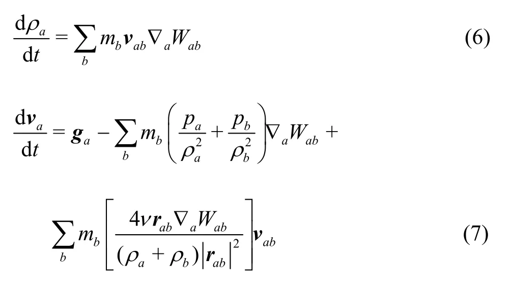
wheredenotes the gradient taken with respect to the coordinates of particlea.

In this study, the fluid phase is treated as weakly compressible where the density in the fluid is allowed to vary slightly. The closure problem is solved by using an equation of state, as a relation between the thepressure andthe density.Following Monaghan[12], the relationship between the pressure and the density for a particleais given bywhere the constantis the reference density,c0is the sound speed at the reference density andγ=7 for a fluid like water. The speed of soundc0is generally chosen as 10 times of the maximum velocity in the fluid to ensure that the fluctuations of the density are less than 1%.

It is a challenging task to implement the solid boundaries in the SPH due to the kernel truncation. In this work, the so-called dynamic boundary conditions[22]are adopted for both the moving and fixed boundaries. This method consists of creating boundary particles that satisfy the same equations of continuity (6) and state (8) as the fluid particles, but without updating their positions using the momentum Eq.(7) and their positions remaining fixed (fixed boundaries) or moving according to some externally imposed function (moving objects).

Finally the particle positions are updated every time-step using the XSPH variant[12]

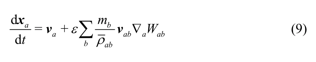
whereandεis a constant, with its value in the range between 0 and 1,ε=0.5, as is often used. This method is a correction for the velocity of a particlea.This correction makes the particles more organized and, for high fluid velocities, helps to avoid the particle penetration.

1.2 Rheological model

The present work simulates the deformable submarine landslide as a non-Newtonian fluid. Generally speaking, the viscosity of incompressible generalized Newtonian fluids depends only on the second principal invariant of the shear strain rate and a classical constitutive law for these generalized Newtonian fluids is in the form

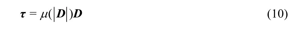
where the shear strain rateand its second invariantThis formulation can also be used to handle visco-plastic fluids.

The Bingham model is one of the simplest model and provides a satisfactory description of the viscoplastic behaviour of the non-Newtonian fluid. A variety of other Bingham models such as the bi-viscosity and Herschel-Bulkley models are often used for submarine sediments to simulate the Bingham rheology of a viscoplastic material in low and high stress states[23]. A bi-viscosity model is a piecewise viscoplastic model using a pseudo-Newtonian viscosity in the un-yielded region and a Bingham viscosity in the yielded region. The Herschel-Bulkley model is a combination of a Bingham model and a power law model. In the Herschel-Bulkley model, as in the Bingham model, no shear stress appears before the yield stress point with a singularity at the point where the shear strain is zero. To avoid this occurrence, Papanastasiou proposed the regularization of the Bingham fluid model by introducing an exponential term, which decreases quickly withwheremis an adjustable parameter, thus smoothing out the viscosity function in a Bingham fluid. With this idea, a model is created, that is valid in both the liquid and solid regions of the material. In the present work, we use the Papanastasiou adaptation for a Herschel-Bulkley fluid, which takes the following form

whereτyandμprepresent the yield stress and the plastic viscosity, respectively, andmis the stress growth exponent. In the limit case ofm→∞, the Herschel-Bulkley model is recovered and hence the choice of the parametermis actually a tradeoff between the numerical issues and the accuracy of the mechanical response. All simulations in this work are performed by usingm=1000s .

1.3 Discrete element method

We use the DEM and the SPH combined to simulate the interaction between the rigid body slides and the viscous free-surface flows. The motion of each slide is tracked based on Newton’s laws of motion as follows:

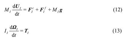
where the massMI, the velocityUI, and the angular velocityΩIare for the solidI, andgis the gravity acceleration. The forceis due to the fluidsolid interaction and the forcerepresents any solid contact that might occur. Integrating Eq.(12) in time advances the linear motion of the solid whereas Eq.(13) accounts for the rotational motion.

In order to calculate the fluid-solid interactionforce, the boundary of a moving solid is represented by groups of SPH particles and these moving boundary particles have an inter-particle spacing equal half of the fluid particle spacing to prevent the fluid particles from penetrating the moving solid boundary. The fluid-solid interaction is ensured through the interactive force balance condition based on the Newton’s third law of motion. Following Ren et al.[13], the fluid-solid interaction forcecan be determined as

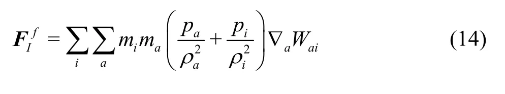
where the inner summation means the total force on a moving boundary particleibelonging to solidIdue to the neighborhood fluid particlea.

Following Latham et al.[24], a multi-sphere approach is used for modeling the complex-shaped multibody dynamics, in which the surface of each solid is represented by a cluster of small spheres of a diameter equivalent to the spacing of the moving boundary particles. The solids are allowed to interact via the contact forces when the surface spheres of different solids overlap. No relative movement between spheres of the same body is allowed. Based on the multi-sphere approach, the resultant contact forces and torque acting upon a solidIare evaluated as

whereRiis the radius of surface sphereibelonging toI,nijrepresents the normal unit vector pointing from the center of sphereibelonging toIto the center of spherejbelonging toJ.fij,nandare the normal and tangential forces, respectively, on surface sphereiof solidIdue to surface spherejof solidJ. The normal contact forcesare calculated by

whereknis the normal spring stiffness, The overlapwhereRiandRjare the surface sphere radii, andxiandxjare the surface sphere centres.vij,nis the normal relative velocity, andηnis the normal damping coefficient given by

whereeijis the restitution coefficient. The effective masswheremiandmjare the masses of surface spheresiandj, respectively.

The tangential component of the contact forceis calculated by a Coulomb friction law using a coefficient of frictionμij. It can be expressed as

wherekt,δtandηtare the tangential spring stiffness, the tangential overlap, and the tangential damping coefficient, respectively. The tangential relative velocityand the tangential unit vectorThe tangential damping coefficient is given by

2. Results and discussions

2.1 Submarine rigid body sliding

As the first numerical validation case, the submerged rigid landslide is investigated in this section. The numerical model used in this simulation is based on a laboratory experiment in literature[16]. In this experiment, the landslide was modeled by a rigid wedge sliding freely into the water along ao45 inclined slope. The cross section of the wedge is an isosceles triangle with a length of 0.5 m. The initial water depth is 1m and the top of the wedge is slightly below the water surface. The initial configuration used in our simulation is shown in Fig.1.

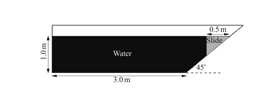
Fig.1 Initial configuration of submerged rigid landslide

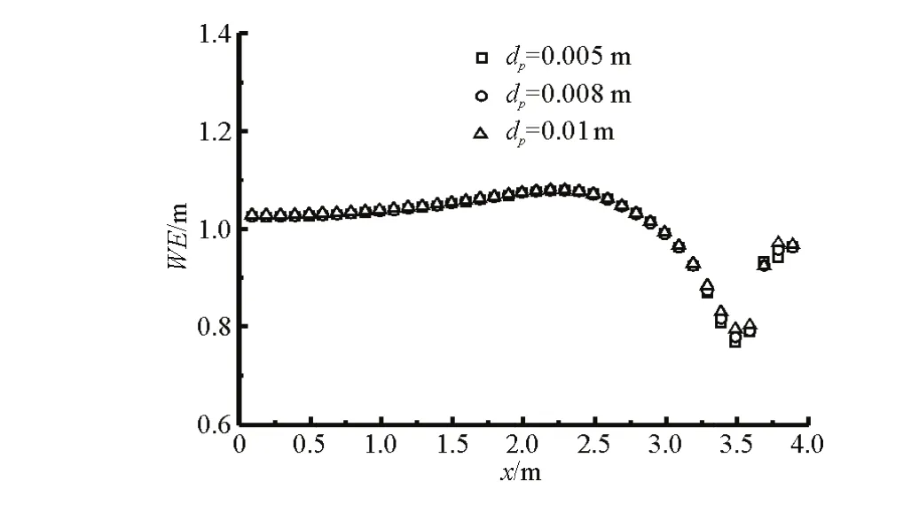
Fig.2 Effect of particle spacing on the accuracy

Fig.3 (Coloronline) Snapshot sequences of the rigid landslide simulation at differen times

The developed SPH-DEM method is applied to the simulation of the submerged rigid landslide process. In this simulation,the modeled fluid is the water of density of 1 000 kg/m3and kinnetic viscosityy of ν=1× 10-6mm2/s .The solid slide has a density of the2 000kg/m3,a normal spring stiffness of 105N/m and a cooefficient of restitution of 0.8. The friction coeffi--ciennt of the conntact face between the sslide and the sloppe was not given inliterature[16].We set the fric--tion coefficient as 0.287 following the work of Wang et al.[2].A time step of 1×10-4s is used in this simu--latioon. In order tto achieve aparticle spaccing indepen--dent solution, the particle spacing is systematically reduced till further reductionn does not allter the solu--tion. Figure 2 shows a typical convergence study with WErepresenting water elevation. Aninitial fluid particle spacingdp=0.01, 00.008 and 0.005 mis usedd for the convergence study and as can be seen that thesolutions for dp =0.008 and dp=0.005are almost the same. A time step of1×10-4s and an initial fluid particle spaccing of 0.005m are usedin the following simulations.The entire coomputation time is 2 s. Figure 3 shows thesubsequent snap shots of the impact water wave at different times by the rigid landslide usingg the coupled SPH-DEM method. The colorbar indicating the velocity magnitudein all snapshots. Figure 4 shows the time history of simulated vertical displacement VD of the rigid slide compared with the experimental results. It is indicated that the numerical computed displacement agrees well with the expperimental displacement, which provesthe accuracyy of the SPH-DEM method in reproducinng the rigid landslide motionn under thesolid-fluidinteraction.The comparison between the numerical and experimental results of the water elevation(WE)profile at times 0.5 s and 1.0 s is shown in Figg.5. From these graphs, we can conclude that the overall behavior of the free surface produced by the SPH-DEM method is in good agrement with the data obtained in the experiment. The comparison indicates that the lanndslide-generated impulsive waves could be simula- teed acurately by using the SPH-DEM method.

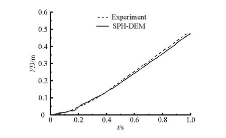
Fig.4 Vertical dispplacement timehistory of the rigid compared with the experiment results

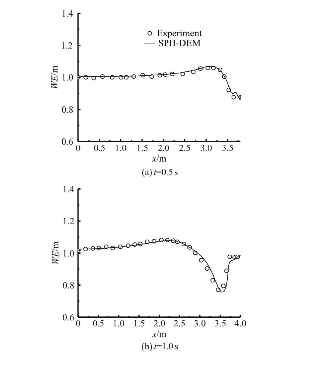
Fig.5 Comparison of the numerically computed water surface with the experimental resultts

Fig.6 Schematic diagram of annular viscometer problem

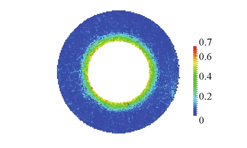
Fig.7 (Color online) A snapshot at t=1s

2.2 SPH modeling of annnular viscometer

In this section, a benchmark problem of the tangential creeping flow in a viscometer made of two coaxial cylinders is studied to demonstrate the cappability of the proposed method to solve non-Newtonian fluid flow problems. As shown in Fig.6, the outer cylinder is kept fixed while the inerr cylinder rotates with a constant angularr velocity ω=1. An initial fluid particle spacing of 0.015 mis used in the computational domain. The time step Δt =1× 10-4s .All material properties are the same as those in literature[25]. Figure 7 showsa snapshot at=1s with the color--barindicating the velocity magnitude. Figure 8 shows the tangential velocities (TV) obtained using the present SPH method and the analytical solutions[25]. It is seen that in this case the solution is in a close agreement with the analytical solution.

Fig.8 Comparison of tangential velocities

2.3 Submarine deformable sand sliding

The SPH-DEM simulation of the submerged rigid landslide is validated in the previous section. In this section, a submerged deformable saand landslidee will be investigated. The numerical model used in this simulation is based on a laboratory experiment in litera--ture[17]. This expperiment consists of generating the water waves by allowing a mass of sand to slide freelyy down a frictionless inclined plane with a slope of 45o(see Fig.9). The channel is 4.00 m long,0.30 m wide and 2.00 m high. The sand mass is as wide as the channel, so that the experiments involve a vertical plane, as a 2-D pproblem. The initial verticcal profile of the sand mass is triangular.This mass is held in its initial position by a vertical guillotine water gate. This gate is lifted up very quicklly at t=0s.The dimen--sions of the cross section of the mass are 0.65 m×0.65 m. The water depth is 1.60 mand the top of the triangular mass is initially 0.1 m below the water surface.

Fig.9 Initial configu ration of submerged deformable landslide

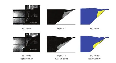
Fig.10 (Color online) Comparison snapshots among results (τy=200 Pa)

In our SPH simulation, the deformable landslide material is approximated as a non-Newtonian fluid. The visco-plastic behaviour of the deformable landslide is modeled by using the Papanastasiou model. In our computations, the density and the kinetic viscosity of the water are 1 000 kg/m3and 1×10-6m2/s, respectively. The mean apparent density of the sand is 1 950 kg/m3. The rheological parameters of the sand were not measured in the experiments but chosen by trials and errors in literature[17]for the numerical simulations. In the simulations of this study, two different rheological coefficients are taken with the yield stress τy=200 Pa and τy=1000 Pa, respectively. In both cases, the viscositypμ is set to 0.002 Pa·s, which is different from the values used in the numerical simulations in literature[17]. This is due to the necessity of our particular rheological model to have a non-zero value for the viscosity, as is indeed the approach used in literature[17]to have an immediate liquefaction of the material. A time step of 1×10-4s and an initial fluid particle spacing of 0.01 m are used in this simulation. The smoothing length is h, defined as 1.2 times of the initial particle spacing. The entire computation time is 1.5 s.

Figure 10 shows the comparison of snapshots among the experiment in literature[17], the previous numerical results in literature[17], and the present SPH results with the yield stress τy=200 Pa at t=0.4 s and 0.8 s. The deformation of the sand sliding and its induced water wave at two different time steps behaves similarly in these three different methods. Comparisons between the experimental and computed water surfaces at t=0.4 s and 0.8 s are shown in Fig.11. It is indicated that the present SPH simulatedresults agree well with experimental results. Figure 12 shows, respectively, the sliding process and the water velocity contour of the submerged sand landslides for the two yield stress values of τy=200 Pa and τy=1000 Pa. In the simulation with a higher value of the yield stressyτ, the sand mass is so rigid that italmost keeps its initial shape. As it can be observed in this graph, the wave amplitude and the slide velocity depend on the yield stress of the sand. The slide with a larger yield stress moves much more slowly and generates smaller waves.

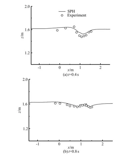
Fig.11 Comparison of experimental and computed water surfaces (τy=200 Pa)

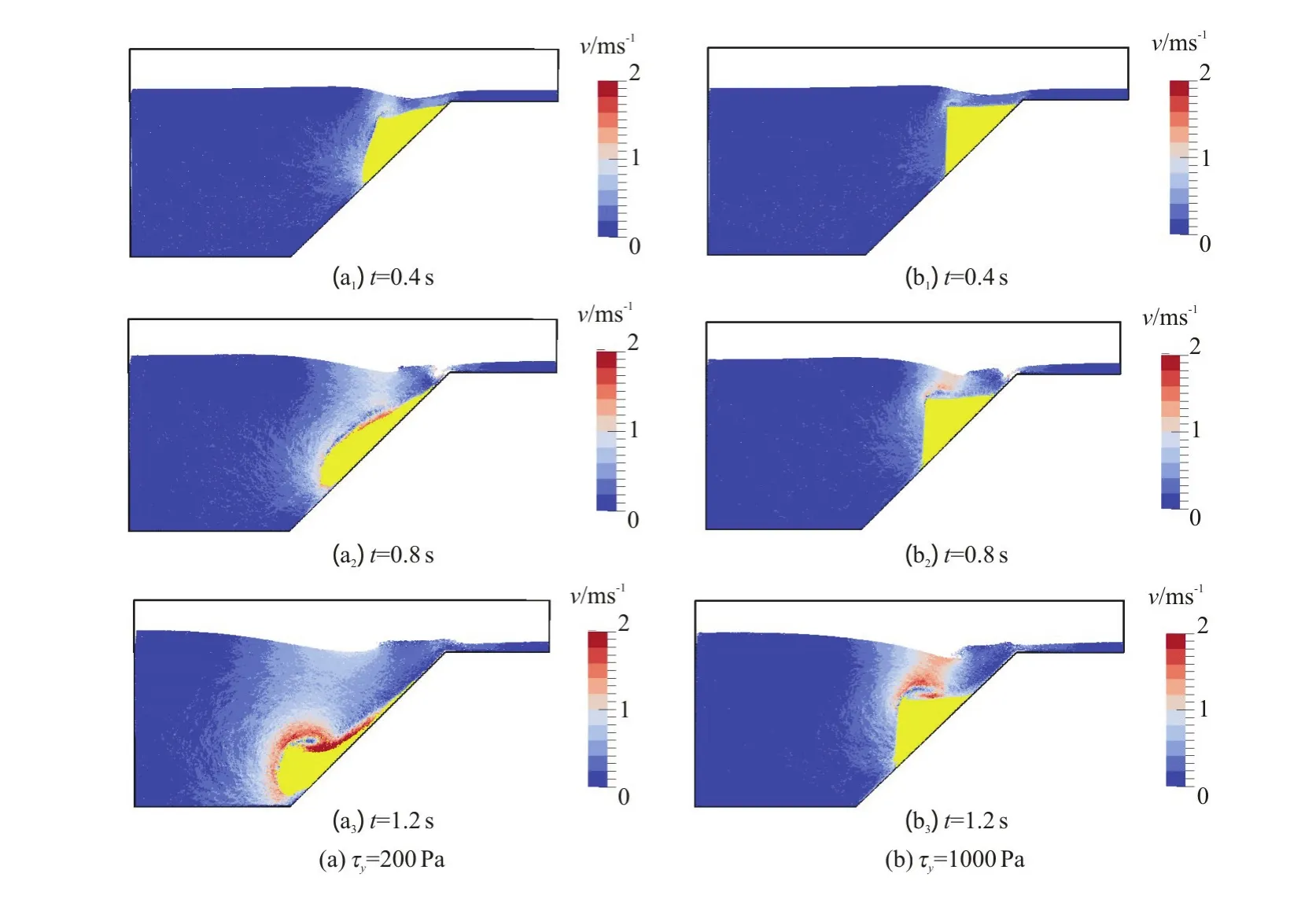
Fig.12 (Color online) Sliding process and water velocity contour of submerged sand landslides

3. Conclusions

We present a particle based method to simulate the full process of the landslide tsunamis due to the rigid and deformable submarine landslides. In this method, a weakly compressible SPH is applied to solve the viscous free surface flow. The movement of the rigid landslides is modeled by using a multi-sphere DEM approach to enable landslides with arbitrarily complex shapes to be modeled. The fluid-solid interaction is simulated by coupling the SPH and the DEM. A rheology model combining the Papanastasiou and the Herschel-Bulkley models is used to represent the viscoplastic characteristics of the non-Newtonian fluid in the deformable landslide simulation. Numerical results are compared with previous scale model experiments of the rigid and deformable landslides to validate the proposed method in terms of accuracy and capability of reproducing the full process of submarine landslides. Good agreement between the numerical solutions and the experimental results is found.

Acknowledgments

This work was supporeted by the Open Fund of the State Key Laboratory of Hydroscience and Engineering of China, Tsinghua University (Grant No. sklhse-2015-C-03), the Open Fund of the State Key Laboratory of Simulation and Regulation of Water Cycle in River Basin, China Institute of Water Resources and Hydropower Research (Grant No. IWHRSKL-201505) and the Open Fund of the State Key Laboratory of Hydraulics and Mountain River Engineering, Sichuan University (Grant No. SKHL1425).

[1] Heller V., Spinneken J. Improved landslide-tsunami prediction: Effects of block model parameters and slide model [J]. Journal of Geophysical Research Oceans, 2013, 118(3): 1489-1507.

[2] Wang W., Chen G. Q., Zhang H. et al. Analysis of landslide-generated impulsive waves using a coupled DDASPH [J]. Engineering Analysis with Boundary Elements, 2016, 64(1): 267-277.

[3] Watts P., Grilli S., Kirby J. et al. Landslide tsunami case studies using a Boussinesq model and a fully nonlinear tsunami generation model [J]. Natural Hazards and Earth System Sciences, 2003, 3(5): 391-402.

[4] Bosa S., Petti M. Shallow water numerical model of the wave generated by the Vajont landslide [J]. Environmental Modelling and Software, 2011, 26(4): 406-18.

[5] Quecedo M., Pastor M., Herreros M. Numerical modelling of impulse wave generated by fast landslides [J]. Interna-tional Journal for Numerical Methods in Engineering, 2004, 59(12): 1633-1656.

[6] Liang D. Evaluating shallow water assumptions in dambreak flows [C]. Proceedings of the Institution of Civil Engineers Water Management, 2010, 163(5): 227-237.

[7] Heidarzadeh M., Krastel S., Yalciner A. C. Submarine mass movements and their consequences (Krastel S., Behrmann J. H., Volker D. et al. Advances in natural and technological hazards research) [M]. New York, USA: Springer, 2014, 37: 483-495.

[8] Zweifel A., Zuccalà D., Gatti D. Comparison between computed and experimentally generated impulse waves [J]. Journal of Hydraulic Engineering, 2007, 133(2): 208-216.

[9] Qiu L. C. Two-dimensional SPH simulations of landslidegenerated water waves [J]. Journal of Hydraulic Engineering, ASCE, 2008,134(5): 668-671.

[10] Fu L., Jin Y. C. Investigation of non-deformable and deformable landslides using meshfree method [J]. Ocean Engineering, 2015, 109: 192-206.

[11] Liu G. R., Liu M. B. Smoothed particle hydrodynamics: A mesh free particle method [M]. Singapore: World Scientific, 2003.

[12] Monaghan J. J. Smoothed particle hydrodynamics [J]. Reports on Progress in Physics, 2005, 68(1): 1703-1759.

[13] Ren B., Jin Z., Gao R. et al. SPH-DEM modeling of the hydraulic stability of 2D blocks on a slope [J]. Journal of Waterway, Port, Coastal, and Ocean Engineering, 2013, 140(6): 1-12.

[14] Canelas R. B., Crespo A. J. C., Dominguez J. M. et al. SPH-DCDEM model for arbitrary geometries in free surface solid-fluid flows [J]. Computer Physics Communications, 2016, 202(1): 131-140.

[15] Cummins S. J., Cleary P. W. Using distributed contacts in DEM[J]. Applied Mathematical Modelling, 2011, 35(4): 1904-1914.

[16] Dong J., Wang B., Liu H. Run-up of non-breaking double solitary waves with equal wave heights on a plane beach [J]. Journal of Hydrodynamics , 2015, 26(6): 939-950.

[17] Qiu L. C. Numerical simulation of water waves generation due to deformable granular landslides [C]. Proceeding of the 11th National Congress on Hydrodynamics and 24th National Conference oh Hydrodynamics and Commemoration of the 110th Anniversary of Zhou Pei-yuanʼs Birth. WuXi, China, 2012,1096-1101.

[18] Macia F., Colagrossi A., Antuono M. et al. Benefits of using a wendland kernel for free-surface flows [C]. 6th International SPHERIC workshop. Hamburg, Germany, 2011, 30-37.

[19] Capone T., Panizzo A., Cecioni C. et al. Accuracy and stability of numerical schemes in SPH [C]. 2nd International SPHERIC Workshop. Madrid, Spain, 2007.

[20] Robinson M. Turbulence and Viscous mixing using smoothed particle hydrodynamics [D]. Doctoral Thesis, Melbourne, Australia: Monash University, 2009.

[21] Lo E., Shao S. Simulation of near-shore solitary wave mechanics by an incompressible SPH method [J]. Applied Ocean Research, 2002, 24(5): 275-286.

[22] Crespo A. J. C., Gómez-Gesteira M., Dalrymple R. A. Boundary conditions generated by dynamic particles in SPH methods [J]. Computers, Materials, and Continua, 2007, 5(3): 173-184.

[23] Jeong S. Determining the viscosity and yield surface of marine sediments using modified Bingham models [J]. Geosciences Journal, 2013,17(3): 241-247.

[24] Latham J. P., Munjiza A., Mindel J. et al. Modelling of massive particulates for breakwater engineering using coupled FEMDEM and CFD [J]. Particuology, 2008, 6(6): 572-583.

[25] Pleiner H., Liu M., Brand H. R. Nonlinear fluid dynamics description of non-Newtonian fluids [J]. Rheologica Acta, 2004, 43(5): 502-508.

(Received July 30 2016, Revised November 30, 2016)

* Project supported by the National Natural Science Foundation of China (Grant Nos. 11172321, 51509248), the Scientific Research and Experiment of Regulation Engineering for the Songhua River Mainstream in Heilongjiang Province (Grant No. SGZL/KY-12).

Biography:Liu-chao Qiu (1971-), Male, Ph. D.,

Associate Professor