Jin-tao Liu (刘锦涛), Peng-cheng Guo (郭鹏程), Tie-jun Chen (陈铁军), Yu-lin Wu (吴玉林)

1. Beijing Institute of Control Engineering, Beijing 100190, China, E-mail: liujintao86@hotmail.com

2. State Key Laboratory Base of Eco-hydraulic Engineering in Arid Area, Xi’an University of Technology, Xi’an 710048, China

3. Department of Thermal Engineeering, Tsinghua University, Beijing 100084, China

The influence of nonlinear shear stress on partially averaged Navier-Stokes (PANS) method*

Jin-tao Liu (刘锦涛)1, Peng-cheng Guo (郭鹏程)2, Tie-jun Chen (陈铁军)2, Yu-lin Wu (吴玉林)3

1. Beijing Institute of Control Engineering, Beijing 100190, China, E-mail: liujintao86@hotmail.com

2. State Key Laboratory Base of Eco-hydraulic Engineering in Arid Area, Xi’an University of Technology, Xi’an 710048, China

3. Department of Thermal Engineeering, Tsinghua University, Beijing 100084, China

2017,29(3):479-484

In most of partially averaged Navier-Stokes (PANS) methods, the Reynolds stress is solved by a linear hypothesis isotropic model. They could not capture all kinds of vortexes in tubomachineries. In this paper, a PANS model is modified from the RNG k-e turbulence model and is used to investigate the influence of the nonlinear shear stress on the simulation of the high pressure gradient flows and the large curvature flows. Comparisons are made between the result obtained by using the PANS model modified from the RNG -ke model and that obtained by using the nonlinear PANS methods. The flow past a curved rectangular duct is calculated by using the PANS methods. The obtained nonlinear shear stress agrees well with the experimental results, especially in the high pressure gradient region. The calculation results show that the nonlinear PANS methods are more reliable than the linear PANS methods for the high pressure gradient flows, the large curvature flows, and they can be used to capture complex vortexes in a turbomachinary.

Nonlinear PANS method, circular cylinder, velocity distribution, unsolved eddy viscosity

Introduction

One way to model the anisotropy is to use the Reynolds stress transport equations. Craft and Launder[1]discussed different Reynolds stress turbulence models and found that higher order pressure strain models with consideration of the stress redistribution near walls can predict the lateral spreading rate well. Lübcke et al.[2]used another way to simulate the anisotropy. They presented an explicit Reynolds-stress closure for a physically sound extension of the most prominent linear Boussinesq viscosity models with a modest computational cost.

Durbin[3]introduced the elliptic relaxation approach within the framework of the linear eddy-visco-sity formulation: the so-called v2-f model. The nonlinear v2-f turbulence model differs from the family of conventional nonlinear eddy viscosity models. In this approach, the elliptic wall effects are accounted for indirectly through the solution of a modified Helmholtz equation[4,5]. The v2-f turbulence model is a seven equation model, which would take more computational time and resources.

The large eddy simulation (LES) may not be computationally viable, due to the large computational cost. Instead, some mixed computational methods, combining the desirable aspects of the RANS and the LES, were used in the engineering computations[6]. Girimaji et al.[7]proposed a new turbulence model that combines the advantages of the RANS method with those of the LES. Girimaji[8]developed a bridging method inspired by the modeling paradigm proposed by Speziale. The method is called the partially averaged Navier-Stokes (PANS) model and is purported for any filter width.

Jeong and Girimaji[9]analyzed the flow past a circular cylinder with a high Reynolds number via thePANS model. Huang and Wang[10]studied the unsteady cavitating flow around the Clark-Y hydrofoil and found that the result agrees well with the experimental result when the unresolved-to-total kinetic energy ( fk) is less than 0.2. Luo et al.[11]and Ji et al.[12,13]analyzed the cavitating flow around a marine propeller and a twisted hydrofoil in a non-uniform wake via the PANS method with the modified -kemodel. Krajnovic et al.[14]studied the flow around a cuboid influenced by the crosswind with a comparison between the PANS model and the LES. Hu et al.[15]proposed a new kind PANS model derived from the k-w turbulence model, which was called the k-wPANS methods. Comparisons between the k-ePANS method and the k-w PANS method were made through simulations of the flow past a circular cylinder by Reyes[16]. A variable-resolved PANS bridging strategy was applied to the four-equation k -e- x- f turbulence model[17]. The k -e -x -f PANS method was more accurate in the simulation of the near-wall turbulence flow. The embedded LES using the PANS model was proposed by Davidson and Peng[18].

Computations of the flow in a curved rectangular duct were also made to evaluate the numerical as well as physical modeling aspects. In this paper, the nonlinear PANS model is used to simulate the flow in a curved rectangular duct. Results of the internal flow are compared with the experimental data.

1. Governing equations

For the incompressible flow, the continuity equation and the Reynolds averaged Navier-Stokes equations are

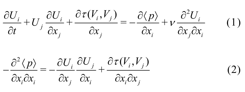
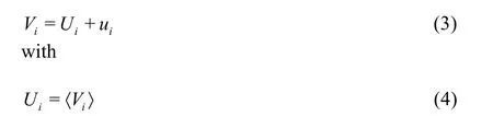
whereiV is the instantaneous velocity (with subscripts i and j indicating the components in different directions), t is the time, p is the pressure, denotes a constant-preserving arbitrary (implicit or explicit) filter commuting with the spatial and temporal differentiations, x denotes the coordinates, n is the kinematic viscosity. Here, Viis partitioned into two parts: the partially averaged velocity (Ui) and the unresolved part (ui)

In the RNG -ke turbulence mode, the equations for the turbulent kinetic energy ()k and the turbulent dissipation ()e can be expressed as follows:

with Cm=0.0845, ak= ae=1.39, Ce1=1.42, Ce2=1.68, h0=4.377, b =0.012. In Eqs.(5) and (6),r is the density,U is the mean component of the velocity, m is the dynamic viscosity, kP denotes the production terms of the turbulence kinetic energy.

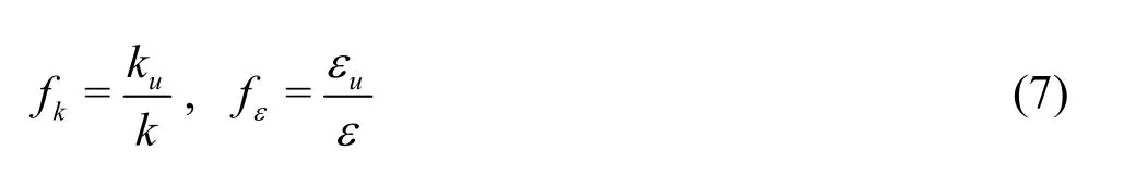
As shown in Girimaji et al.[7], the extent of the PANS averaging relative to the RANS can be quantified by using the unresolved-to-total ratios of the kinetic energy (fk) and the dissipations ( fe)

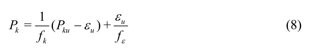
The relationship betweenkP in the RNG -keturbulence mode andkuP in the PANS model can obtained through comparing the source terms such as

Then we can obtain the PANS model by a modification of the RNG -ke turbulence model with thefollow in g equations:

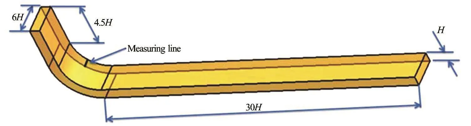
Fig.1 (Color online) A curved rectangular duct

Equations (9) and (10) form the linear PANS model.

The shear stress is solved by using the nonlinear turbulence model proposed by Liu et al.[19]:

In Eq.(15), T is the turbulence time scale and u is the turbulence velocity scale.

The use of the nonlinear shear stress in the linear PANS model makes the nonlinear PANS model.

2. Test case

To show that the nonlinear PANS can be used for capturing complex flows, a 3-D curved rectangular duct and the flow past a circular cylinder are simulated and the results of the internal flow are compared with the experimental data. The nonlinear PANS and linear PANS models are implemented with the Fluent software and the user defined function (UDF). The computational results of the nonlinear PANS model are also compared with the results obtained by using the linear PANS model.

The experimental data of the internal flow in the curved rectangular duct were obtained by Kim and Patel[20]. The structure of the curved rectangular duct is shown in Fig.1. H =0.203m , the radius of theinner circle is 0.608 m, and the Reynolds number is Re=u0H /n =2.24´ 105. The transverse velocity (perpendicular to the measurement line and along the flow direction), the axial velocity (perpendicular to the measurement line and the flow direction) and the longitudinal velocity (along the measurement line) on the measurement curve are calculated. Mesh of the rectangular duct is shown in Fig.2.

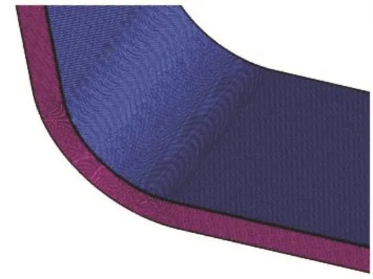
Fig.2 (Color online) Mesh of the rectangular duct

The velocity inlet and the pressure outlet are used. No slip boundary conditions are used for the near wall region. The coupling method is used to correct the pressure during the calculation. The second order upwind scheme is used to resolve the Navies-Stocks equations. Convergence is determined by the residual error less than 0.0001.

3. Results and discussions

3.1 Velocity distribution on the measurement line

Figure 3 shows the results of the transverse velocity on the measurement line. The results obtained by using the nonlinear PANS model with fk=0.1 are in good agreement with the experimental results. The transverse velocity of the experimental results on the measurement line shows a hump shape distribution, and it can be captured by the nonlinear PANS model when fk=0.1. The results obtained by using the nonlinear PANS model with fk=0.2 and the linear PANS model with fk=0.1do not show the nonlinear phenomena.

Fig.3 Transverse velocity

Figure 4 shows the longitudinal velocity on the measurement line. The results obtained by using the nonlinear PANS and the linear PANS model with fk=0.1 are smaller than those obtained by using the nonlinear PANS model with fk=0.2 at the region of the dominant flow. The longitudinal velocity on the measurement line based on the nonlinear PANS model with fk=0.1 agrees well with the experiment result. The results of the longitudinal velocity obtained by using the nonlinear PANS model with fk=0.1 show the nonlinear phenomena when 0＜h/H＜0.3 .

Fig.4 Longitudinal velocity

Figure 5 shows the axial velocity on the measurement line. The maximum point of the axial velocity obtained by using the nonlinear PANS model with fk=0.1 is very close to the result of the experimental data, while the results based on the nonlinear PANS model with fk=0.2and the linear PANS model with fk=0.1 see a large error at this point. The nonlinear characteristics of the axial velocity when 0＜h/H＜0.3 can also be captured by the nonlinear PANS model.

Fig.5 Axial velocity

3.2 Pressure and velocity distributions on the convex surface

The pressure distributions on the convex surface of the curved rectangular duct are shown in Fig.6. The results based on the nonlinear PANS model see a large region of negative pressure, while the results obtainedby using the linear PANS model with fk=0.1 can only capture a small region of negative pressure. Results of the nonlinear PANS model are much different from those of the linear PANS model. The nonlinear PANS model can capture the high pressure gradient on the convex surface.

Fig.6 (Color online) Pressure distribution on the convex surface

3.3 Limit streamline near the convex surface

Figure 7 shows the results of the limit streamline near the convex surface. Results of the RNG -kemodel and the SST -kw model see flow separation phenomena, as shown in Fig.8(b). The flow also has a symmetric distribution without vortex near the convex surface, as obtained by using the RNG -ke model and the SST -kw model. The results of the limit streamline near the convex surface based on the nonlinear PANS model see a great difference from those obtained by using the other two models. Both the flow separation and the reverse flow can be captured by the nonlinear PANS model. The flow separation at the front of the curved rectangular duct is the same as that obtained by using the other turbulence model, but the results of the RNG -ke model and the SST -kwmodel do not see the reverse flow at the curved region.

Fig.7 Velocity distribution on the convex surface

4. Conclusions

This paper investigates a nonlinear PANS turbulence model and a linear PANS turbulence model, including a sensitivity analysis of the high pressure gradient flow and the large curvature flow. The differencebetween the nonlinear PANS model and linear PANS model is in the use of the nonlinear shear stress.

Results for the curved rectangular duct indicate that the nonlinear shear stress shows a nontrivial improvement compared with the linear PANS model. Results of the velocity on the measurement line based on the nonlinear PANS model with fk=0.1 are in good agreement with the experimental results. The model using the nonlinear shear stress can capture the flow separation and the reverse flow.

Acknowledgment

This work was supported by the Open Research Fund Program of State Key Laboratory of Hydroscience and Engineering, Tsinghua University (Grant No. sklhse-2014-E-02).

[1] Craft T. J., Launder B. E. On the spreading mechanism of the three-dimensional turbulent wall jet [J]. Journal of Fluid Mechanics, 2001, 435: 305-326.

[2] Lübcke H. M., Rung T., Thiele F. Prediction of the spreading mechanism of 3D turbulent wall jets with explicit Reynolds-stress closure [J]. International Journal of Heat and Fluid Flow, 2003, 24(4): 434-443.

[3] Durbin P. Separated flow computations with the k -e-v2model [J]. AIAA Journal, 1995, 33(4): 659-664.

[4] Laurence D. R., Uribe J. C., Utyuzhnikov S. V. A robust formulation of the v2-f model [J]. Flow Turbulence and Combustion, 2005, 73(3): 169-185.

[5] Popovac M., Hanjalic K. Compound wall treatment for RANS computation of complex turbulent flows and heat transfer [J]. Flow Turbulence and Combustion, 2007, 78(2): 177-202.

[6] Tucker P. G. Trends in turbomachinery turbulence treatments [J]. Progress in Aerospace Sciences, 2013, 63(6): 1-32.

[7] Girimaji S. S., Jeong E., Srinivasan R. Partially averaged Navier-Stokes method for turbulence: Fixed point analysis and comparison with unsteady partially averaged Navier-Stokes [J]. Journal of Applied Mechanics, 2006, 73(3): 422-429.

[8] Girimaji S. S. Partially-averaged Navier-Stokes model for turbulence: A Reynolds-averaged Navier-Stokes to direct numerical simulation bridging method [J]. Journal of Applied Mechanics, 2006, 73(3): 413-421.

[9] Jeong E., Girimaji S. S. Partially averaged Navier-Stokes (PANS) method for turbulence simulations-Flow past a square cylinder [J]. Journal of Fluids Engineering, 2010, 132(12): 121203.

[10] Huang B., Wang G. Y. Partially averaged Navier-Stokes method for time-dependent turbulent cavitating flows [J]. Journal of Hydrodynamics, 2011, 23(1): 26-33.

[11] Luo X. W., Ji B., Tsujimoto Y. A review of cavitation in hydraulic machinery [J]. Journal of Hydrodynamics, 2016, 28(3): 335-358.

[12] Ji B., Luo X. W., Wu Y . L. et al. Partially-averaged Navier-Stokes method with modified -kemodel for cavitating flow around a marine propeller in a non-uniform wake [J]. International Journal of Heat and Mass Transfer, 2012, 55(23-24): 6582-6588.

[13] Ji B., Luo X., Wu Y. et al. Numerical analysis of unsteady cavitating turbulent flow and shedding horse-shoe vortex structure around a twisted hydrofoil [J]. International Journal of Multiphase Flow, 2013, 51(5): 33-43.

[14] Krajnovic S., Ringqvist P., Basara B. Comparison of partially averaged Navier-Stokes and large-eddy simulations of the flow around a cuboid influenced by crosswind [J]. Journal of Fluids Engineering, 2012, 134(10): 101202.

[15] Hu C. L., Wang G. Y., Wang Z. Y. Partially averaged Navier-Stokes method based on -kw model for simulating unsteady cavitating flows [J]. Materials Science and Engineering, 2015, 72(2): 022007.

[16] Reyes D. A. Partially averaged Navier-Stokes turbulence modeling: Investigation of computational and physical closure issues in flow past a circular cylinder [D]. Master Thesis, College Station, USA: Texas A&M University, 2006.

[17] Basara B., Krajnović S., Girimaji S. et al. Near-wall formulation of the partially averaged Navier-Stokes turbulence model [J]. AIAA Journal, 2011, 49(12): 2627-2636.

[18] Davidson L., Peng S. H. Embedded large-eddy simulation using the partially averaged Navier-Stokes model [J]. AIAA Journal, 2013, 51(5): 1066-1079.

[19] Liu J., Zuo Z., Wu Y. et al. A nonlinear partially-averaged Navier-Stokes model for turbulence [J]. Computers and Fluids, 2014,102(10): 32-40.

[20] Kim W. J., Patel V. C. An experimental study of boundary layer flow in a curved rectangular duct [C]. Proceedings of the ASME Fluids Engineering Conference. Washington DC, USA, 1993.

10.1016/S1001-6058(16)60759-X

May 16, 2015, Revised November 22, 2015)

* Project supported by the National Natural Science Foundation of China (Grant Nos. 51406010, 51479166).

Biography:Jin-tao Liu (1986-), Male, Ph. D., Senior Engineer

Peng-cheng Guo,

E-mail: guoyicheng@xaut.edu.cn