Pengcheng MU (穆鹏程)

School of Mathematics and Statistics, Northeast Normal University, Changchun 130024, China E-mail : mupc288@nenu.edu.cn

Qiangchang JU (琚 强昌)†

Institute of Applied Physics and Computational Mathematics, Beijing 100088, China E-mail : ju qiangchang@iapcm.ac.cn

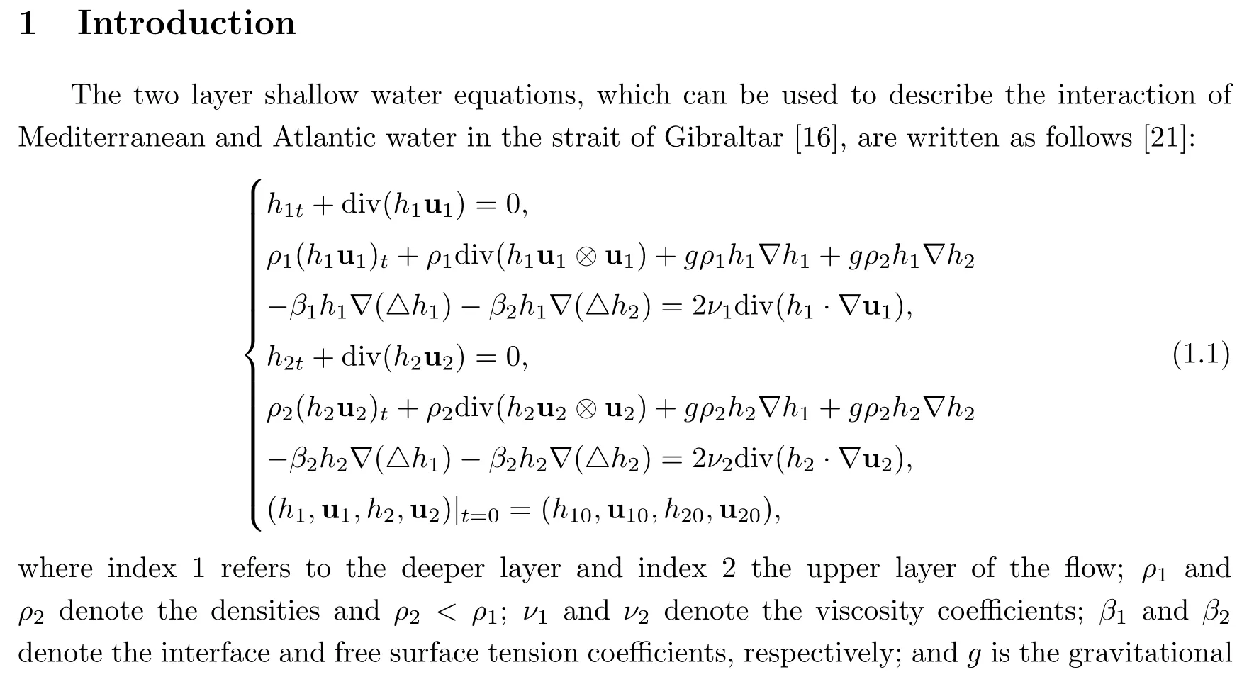
acceleration.All of these physical coefficients are positive constants.hj=hj(t,x)anduj=uj(t,x)denote the thickness and velocity field of each layer,wherej=1,2.

Distinguished from the single layer model,the two layer shallow water equations capture something of the density stratification of the ocean,and it is a powerful model of many geophysically interesting phenomena,as well as being physically realizable in the laboratory[4,9,19].However,there are only a few mathematical analyse of the two layer model.Zabsonr´e-Reina[21]obtained the existence of global weak solutions in a periodic domain and Roamba-Zabsonr´e[18]proved the global existence of weak solutions for the two layer viscous shallow water equations without friction or capillary term.There are other results regarding weak solutions of the two layer shallow water equations in[10,15].To the best of our knowledge,there are no results about the strong solution to the 2-D two layer viscous shallow water equations.In the present paper,our aim is to prove the existence and uniqueness of the global strong solution of(1.1)in the whole spacex∈R2.

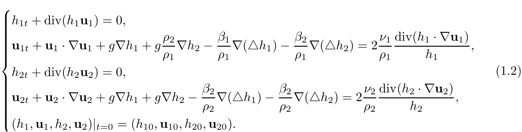
Dividing the second and the fourth equations in(1.1)byρ1h1andρ2h2,respectively,we have

We seek the solution of(1.2)near the equilibrium state(h1,u1,h2,u2)=(1,0,1,0).To this end,putting the transformhj=1+hj0=1+,j=1,2 into the above equations,and dropping the tilde,we have

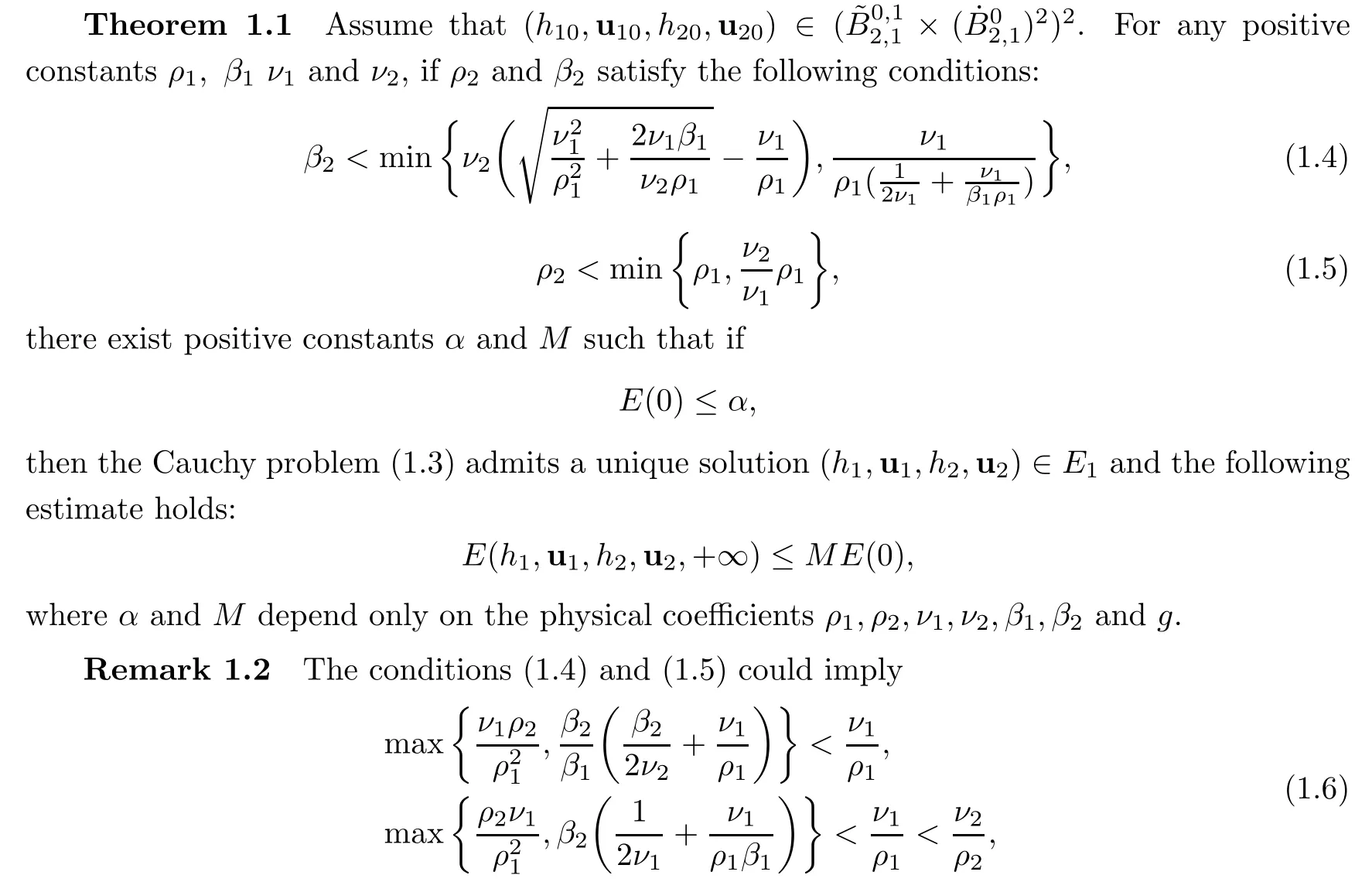
Now we state the main result of this paper.For convenience,we set

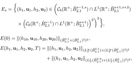
where Cb(R+;X)is the subset of functions ofL∞(R+;X)which are continuous and bounded on R+with values inXandLpT(X)=Lp(0,T;X).Then we have

which are used to deal with the linear terms in the a priori estimates in Section 3.2.

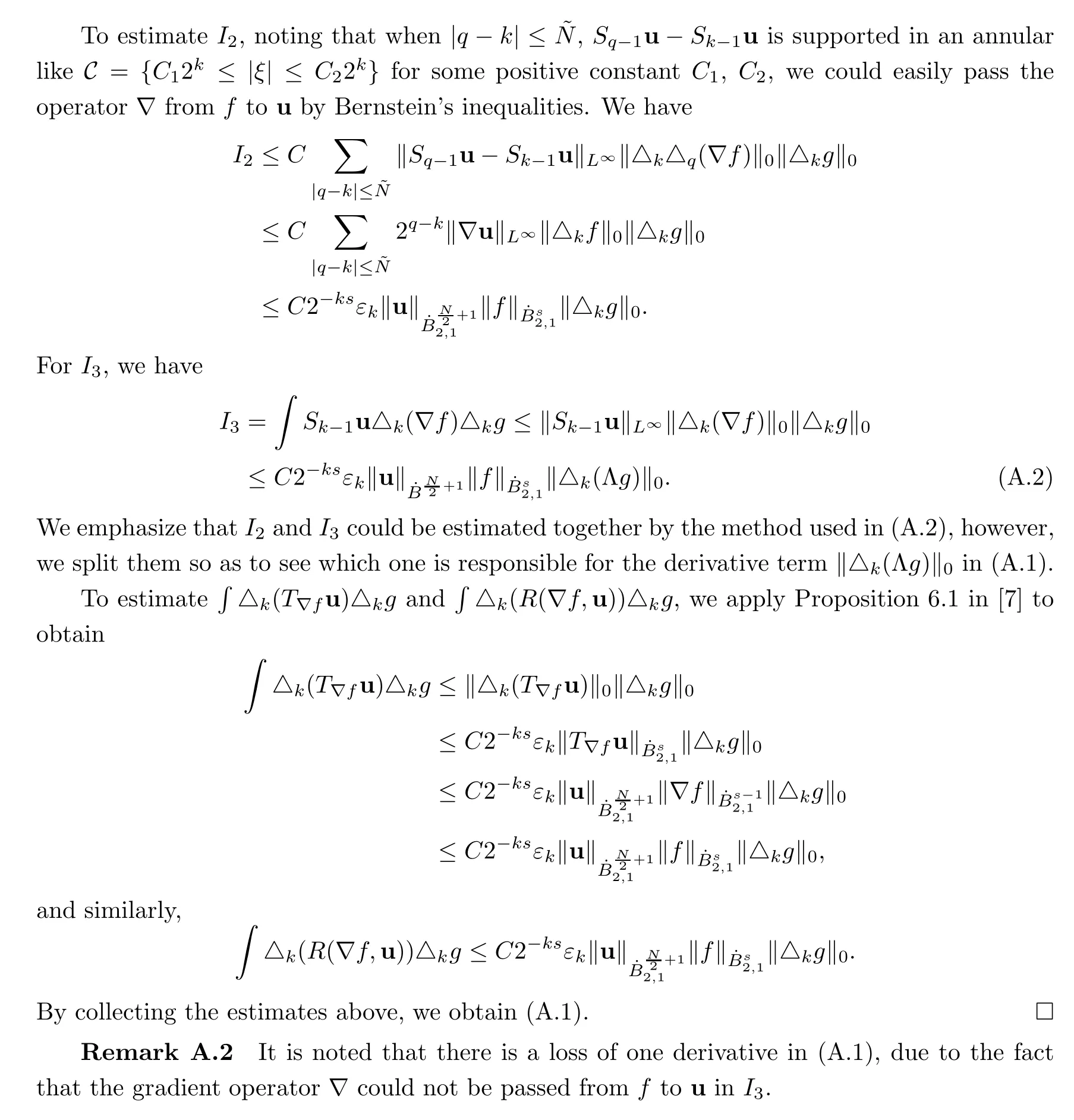
In the proof of Theorem 1.1,the main difficulties arise from the complexity of the system and the coupling of pressure terms in momentum equations.We could not directly split the system into the two independent parts,and the method for the single layer shallow water equations in[12,13]couldn’t work in our case.To dispose of the coupling,we perform a careful combination of the elementary estimates(see(3.19)).However,some other nonlinear coupling terms appear in the new combination estimates for which Lemma 6.2 in[7],used in[3,12,13]to deal with the convection terms in single layer shallow water system,cannot be applied.Therefore,we construct a proposition in the Appendix to estimate these troublesome terms in our problem,which is a standard generalization of Lemma 6.2 in[7].

In this paper,the Littlewood-Paley decomposition will be used to construct the a priori estimates in a hybrid Besov space and the solution of(1.3)is obtained by the Friedrichs’regularization method.Finally,the uniqueness of the solution will be proved directly with the help of the estimates we construct.Some ideas of this paper are motivated by Danchin[6].

We also mention some results regarding the Cauchy problem for the 2-D single layer shallow water equations.For example,Wang-Xu[20]obtained the local solution for any initial data and obtained the global solution for small initial data in Sobolev spaceH2+s(R2)withs>0.Then,Chen-Miao-Zhang[3]improved the result of Wang-Xu by getting the global existence in time for small initial dataIn[13],Haspot considered the compressible Navier-Stokes equation with density dependent viscosity coefficients and a term of capillarity,and obtained the global existence and uniqueness in critical space.In[12],Hao-Hsiao-Li studied the single layer viscous equations with both rotation and capillary term,and also obtained the global well-posedness in Besov space.In addition,there are some researchs on the global weak solutions of the single layer shallow water equations in[2,11,14].Other results related to the regularities of the oceanic flow can be found in[5,17].

The paper is arranged as follows:in Section 2 we recall the definitions and some properties of Besov spaces;in Section 3 we give the a priori estimates of the linear system of(1.3)in a hybrid Besov space;in Section 4 we prove Theorem 1.1 by the classical Friedrichs’regularization method.Finally in appendix we give a proposition that is used in this paper.

2 Littlewood-Paley Theory and Besov Spaces

In this section,we recall the definitions and some properties of Littlewood-Paley decomposition and Besov spaces.The details can be found in[1,7,8].

2.1 Littlewood-Paley decomposition

However,the right-hand side in(2.1)does not necessarily converge in S′(RN).Even if it does,the equality is not always true in S′(RN)(consider the caseu=1).Hence we will define the homogeneous Besov spaces in the following way:

2.2 Homogenous Besov spaces

2.3 Hybrid Besov spaces

In this paper,we will use the following hybrid Besov spaces:

Definition 2.4Lets,t∈R,1≤p,r≤+∞,and define

2.4 Some estimates

The action of some smooth functions on Besov spaces is involved in the following proposition[7].

3 A Priori Estimates

3.1 Preparation for the estimates

Letcj=Λ−1divuj,dj=Λ−1div⊥uj,where div⊥uj=∇⊥·uj,∇⊥=(−∂2,∂1)andΛ−1is defined in Section 2.4.It is easy to check that

For convenience,we set

3.2 Estimates of linear terms

By H¨older’s inequality,we have

3.3 Estimates of nonlinear terms

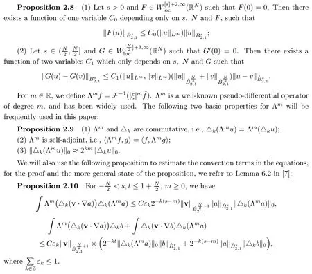
Now we estimate the nonlinear terms inNk.Assume thats∈(0,2].We are not going to estimate all of the terms inNk,but only some of them.For example,by Proposition 2.3,Proposition 2.9 and Proposition 2.10,we have

3.4 Accomplishment of the proof of Proposition 3.1

4 Existence and Uniqueness

With Proposition 3.1 in hand,we can prove the existence of the solution of(1.3)through the classical Friedrichs’regularization method,which was used in[12,13]and the references therein.

4.1 Construction of the approximate solutions

Define the operators{Jn}n∈Nby

4.2 Uniform estimates

Appendix

This section is devoted to proving a proposition which is a supplement of Lemma 6.2 in[7]and has been used in Section 3.We need the following Bony’s decomposition(modulo a polynomial):