YU Kai-bor, FENNDEZ Manuel F

(1. Shanghai Key Laboratory of Intelligent Sensing and Recognition,Shanghai Jiao Tong University， Shanghai 200240, China) (2. Syracuse University, New York 13035, USA)

·DBF在现代雷达中的应用·

Deterministic Nulling for Antenna Pattern of Digital Beamforming Radar Systems

YU Kai-bor1, FENNDEZ Manuel F2

(1. Shanghai Key Laboratory of Intelligent Sensing and Recognition,Shanghai Jiao Tong University， Shanghai 200240, China) (2. Syracuse University, New York 13035, USA)

Deterministic nulling arises in digital beamforming radar applications where the locations of interferers and clutter regions are either known a-priori or can be determined by other means. We address this problem of deterministic nulling by specifying the resulting antenna patterns with multiple nulls that include those extending continuously across intervals of prescribed widths. The solution involves determining the basis vectors for the null spaces of such extended regions, or their composite, via the singular value decomposition of the pertinent portions of the antenna response matrix. An efficient practical implementation of this procedure is then provided.

antenna pattern; array beamforming; array response matrix; null-space; blocking matrix; discrete nulls; extended nulls; mixed-matrix; quiescent pattern

0 Introduction

Inserting nulls in an antenna beam pattern is a problem of interest in radar, sonar and sensor array applications where the locations of interferers and clutter regions are either known a-priori or can be determined by other means[1-5]. An approach for affecting such null insertion involves the use of a “blocking matrix” projecting the beamforming weight vector of interest into the space defined by the set of basis vectors orthogonal to that of the region to be nulled. This approach has the attractive feature of involving a simple modification of the antenna beamforming weights chosen per the particulars of the application of concern.

The techniques for inserting multiple discrete nulls while largely maintaining a desired quiescent beam pat-tern are well-known (reviewedandsummarizedinSection1),while the technique for inserting a broad null can be formulated as a quadratic constraint problem with a solution characterized by the principal eigenvectors of the correlation matrix of the continuum of look-directions defining such null[6]. In this paper we extend the problem to that concerned with inserting both, multiple discrete and multiple broad continuous nulls, and introduce for this purpose the use of quasi-matrices and their factorizations[7]. The resulting solution is further refined as in [8], using a low-rank approximation to balance the null-depth and the pattern distortion. An efficient implementation procedure based on pre-determined basis vectors for various null-widths is then developed.

Section 1 reviews and summarizes the solution for the deterministic nulling problem of the digital beamforming (DBF) radar system which is formulated as a DBF problem with a prescribed number of discrete nulls. The solution involves a least squares (LS) problem with constraints suppressing (“blocking”) the slices of the anten-

na array response corresponding to the spatial directions that are to be nulled.

In Section 2, the problem of deterministic nulling for DBF with continuous extended nulls is formulated. The constraint in this case corresponds to one or multiple spatial regions of the antenna array response; in other words, to a quasi-matrix, a matrix-like construct that is continuous in one dimension (the spatial) and discrete along the other (antenna element)[9]. A way to approach such continuous problem involves discretizing the sources over the constraint extent to then employ the techniques developed for discrete sources discussed in Section 2. Otherwise, an exact approach involves forming the correlation matrix over the continuous sources, as the result is a classical matrix of finite dimension and its eigenvalue decomposition can be used to determine the null space. Alternatively, since the resulting correlation matrix is highly ill-conditioned, the continuous wide-null problem may be approached in a numerically more robust fashion by using quasi-matrix factorization algorithms.

In Section 3 we give a brief overview of quasi-matrices and related factorization algorithms. We then prescribe an algorithm for obtaining the singular value decomposition (SVD) of the continuously-defined antenna response quasi-matrix which involves forming the QR decomposition using modified Gram Schmidt (MGS) transformations[10-11]. Another approach is to directly generate the extended null′s basis vectors using the MGS procedure with column pivoting.

Section 4 uses simulation examples to illustrate the techniques for the continuous extended null-insertion problem using the quasi-matrix approach, and show the trade-offs involved between null-depth and pattern distortion.

Section 5 presents an efficient implementation procedure using pre-determined sets of basis vectors for different null widths. Simulations illustrate the efficiency of this approach for inserting multiple discrete and continuous nulls.

Section 6 summarizes our results.

1 Deterministic Nulling Problem of DBF Radar

(1)

whereu= sin(Θ),Θis the direction-of-arrival angle, andnis the antenna element index. In many applications it is desired to form nulls at discrete directionsuk,k= 1, 2, …,K; that is,

(2)

The nulls may correspond to radio frequency interference (RFI) and discrete clutter with known locations. The null insertion process can thus be formulated as

(3)

whereGis the antenna array response matrix to the desired null directions given by the following

(4)

(5)

which results in

wq-GH(GGH)-1Gwq

(6)

Notice that the matrix operating onwq, namely

(7)

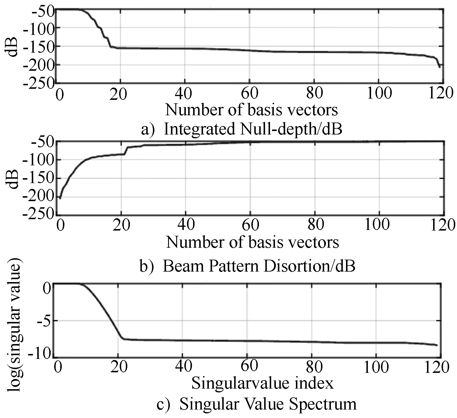
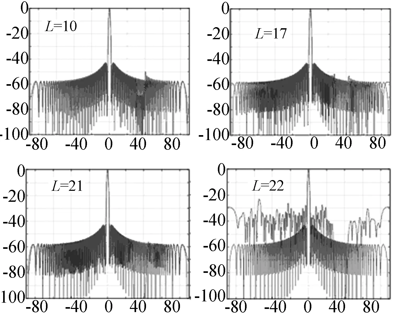
Direct implementation of solution (6) involves inverting theK×KHermitian matrixGGH, which whenK<

GH=Q[RH∶0T]H

(8)

whereQis aK×Kunitary matrix (i.e.,QHQ=QQH=I),Ris anN×Nupper-triangular matrix, and 0 is a (K-N)×Nzero matrix. Note that substituting (8) in (6) yields

(9)

When the conditionK<N), requiring making provisions in the algorithm implementation to handle such eventuality. The most stable approach (albeit computationally the costliest) involves computing the SVD ofG

G =USVH

(10)

where theK×KmatrixUand theN×NmatrixVare unitary, and theK×NmatrixSis diagonal with non-negative diagonal elements arranged in a non-ascending order[10]. WhenGis ill-conditioned, one may set to zero those elements ofSfalling below a thresholdτselected based on criterions to be discussed in the following sections of this paper. Expression (10) can then be expressed as

(11)

where theL×Lnon-negative diagonal matrixS1contains the elements ofSexceedingτ(Lis the rank ofG),U1andU2respectively represent the firstLand lastK-Lcol-umns ofU, andV1andV2represent the firstLand lastN-Lcolumns ofV. One can verify that

(12)

The modified weight vector can thus be obtained using eitherV1or byV2, as convenient; that is,

(13)

ItshouldbenotedthatthematrixVofrightsingularvectorsVcanalsobedeterminedfromtheeigenvaluedecompositionthecorrelationmatrix

GHG = V S2VH

(14)

whereSandVare as previously defined for expression (10). Algorithms exist that exploit the fact that correlation matrices are Hermitian to compute the eigenvalue decomposition in (14) more efficiently[10], although as will be seen later, particular care may be required as, in the particular case of (14), the problem will be rank-deficient or, in the case of extended nulls, highly ill-conditioned. Anyway, once the decomposition is effected, the null space is determined by the eigenvectors corresponding to the zero or “near-zero” eigenvalues. In practice, as in the case of (11), such eigenvalues are determined by some thresholding procedure.

It should be noted that a numerically more stable solution than (14) involves computing the QR-decomposition with column pivoting[10]ofGH; that is

(15)

SplittingQas [Q1∶Q2] yields

GH=[Q1∶Q2][RH∶0T]HP

(16)

whereQ1andQ2now denote respectively the firstLand the lastK-Lcolumns of matrixQ. Ideally, matricesQiare related to theViin (11) asVi=QiTi, where theTiare square unitary transformations, thus enabling expressing (13) using the sets of basis vectorsQ1and/orQ2via

(17)

This yields an algorithm that is far cheaper to implement than either (11) or (14), as well as numerically more stable than (6) and (14), as no correlation matrix is involved; however, determining the rankLofGvia the QR decomposition may not be as accurate as that provided by the SVD.

WhenK>N, as may be the case when modeling extended continuous nulls (see Section 2), computation of the QR-decomposition ofG, followed by the SVD of the resultingR, yields a computational efficient and numerically stable procedure for obtaining the matrixVcontaining the desired sets of range and null basis vectors. In such case, albeitGwill likely be extremely ill-conditioned, obtaining its range and null basis will technically require thresholding the singular values ofR; that is

G=Q[RH∶0T]H≈Q[(U[S∶0T]TVH)H∶0T]T

(18)

whereQisK×K,UandVareN×N, andSisL×L, withLthe estimated rank ofG. MatrixVcan now be split asV=[V1∶V2], withV1(N×L) andV2(N×(N-L)) respectively containing the basis vectors for the range and null spaces ofG(observe that explicit computation ofQis not needed).

In summary, for a set of discrete nulls, the following algorithms can be used to determine the modified weight vector resulting from a constrained LS minimization problem: (a) direct computation of the projection operator as in (6); (b) obtaining the projection operator in terms of theQmatrix from the QR-decomposition ofGH(as in (8) or (15)); (c) computation of the range and null-space basis vectors ofGvia the SVD (expressions (11) or (18)); and (d) computation of the null-space basis vectors ofGvia the eigenvalue decomposition (EVD) ofGGH(14).

(19)

Unfortunately, as shown in the example of Section 4, the pattern nulls produced by such direct LS solution are extremely shallow.

2 Continuous Wide Null Insertion

Consider inserting a continuous, extended null in a sine-space region bounded byua≤u≤ub. This is often done not only to suppress extended sources of clutter or interference, but also to provide robust procedures that account for moving sources and/or sensors, as well as for uncertainties in prior direction or angle estimates. The correspondingGfor such null is called a quasi-matrix of dimension [ua,ub]×Nwhere each column is an element response function continuously defined on interval [ua,ub].

One convenient approach to addressing this continuous problem is to approximate the extended nulls by inserting discrete nulls at multiple, closely-spaced look directions. The techniques discussed in Section 1 for discrete null insertion can then be applied. However, issues with this method are the possibilities of inadequate null-depth and of “leakage” (i.e., of lacking enough suppression in the spaces between discrete nulls) when not enough discrete sources are modeled.

When modeling continuous nulls as a number of discrete sources, the number of rows of the corresponding constraint matrixGmay be relatively large compared to the number of antenna elements, perhaps even exceeding it for the case of large extended nulls. In such cases, the algorithm described by Expression (18) can be used to obtain the proper sets of basis vectors.

The same situation carries over to the continuous null case, when the antenna null response is a quasi-matrixG(u). An overview of quasi-matrices including their factorization is addressed in Section 3, so we will address here the problem by considering instead theN×Ncorrelation matrixPGresulting from the quasi-matrix product

PG=G(u)HG(u)

(20)

with (m,n)thelement given by the following

我们在田里对话就像家中一般平常，几乎忘记是站在庞大的雨阵中，母亲大概是看到我愣头愣脑的样子，笑了，说：“打在头上会痛吧！”然后顺手割下一片最大的芋叶，让我撑着，芋叶遮不住西北雨，却可以暂时挡住雨的疼痛。

(21)

Note that this can be written in matrix form as

(22)

whereDis theN×Ndiagonal unitary matrix of phases

D=diag(ejπ(n-1)uc), n=1,2,…,N

(23)

m=1,2,…,N；n=1,2,…,N

(24)

with

uc=(ua+ub)/2

(25)

and

W=ub-ua

(26)

That is,ucis the center point of the null in sine space, whileWdenotes the desired null width, also in sine space. Therefore

(27)

(28)

(29)

The IND improves with increasingL; that is, null-depth will increase as our approximation uses more and more of the singular values ofG. On the other hand, increasingLwill increase beam pattern distortion (PD) as defined by

(30)

For the continuous extended null case, the singular values can be determined by computing the SVD of quasi-matrix G(u) (this is addressed in Section 3) or they can be derived from the EVD of the correlation matrix given by (21).

3 Quasi-matrix Model for Continuous Nulls

In this section, we first give an overview of the quasi-matrix concept and then prescribe an algorithm to obtain the SVD of G(u), which can be used for solving the continuous null insertion problem.

As described in [7, 9, 11, 13-14], quasi-matrices are arrays whose columns are comprised of continuous functions. This means they lack individual rows in the usual “matrix” sense of the word, thus differing from classical matrices, even those with an infinite number of rows. The term “quasi-matrix” was coined by Stewart[9], who proposed using such constructs to bridge the fields of matrix and approximation theory, hence enabling the latter to exploit the former’s simplicity of notation and its rich trove of data transformations.

The dimensions of a quasi-matrix with N columns consisting of functions defined over interval [ua,ub] is said to be [ua,ub]×N[11]. Notice that vertically stacking conventional matrices and quasi-matrices is perfectly acceptable as long as they all have the same number of columns. This stacking yields “mixed-matrices” that, from the application and implementation perspectives, are far more general and practical than the individual blocks, as they enable exploiting the properties of the two array types (e.g., mixed-matrices can be used to specify both, multiple discrete and extended nulls).

The inner-product of two quasi-vectors x(u) and y(u), specified over interval u in [a, b], is the definite integral of the direct product of the underlying functions x(u) and y(u); thus

(31)

Thisdefinitionenablestranslating,withminorvariations,thematrixdecompositionalgorithmsofSection1toencompassmixed-andquasi-matrices.Themostseamlesswaytoperformquasi-matrixQR-typedecompositionsinvolvesusingtheMGSdecompositionmethod[11,13];infact,attemptsatextendingtoquasi-matricesothercommonmatrixQR-decompositiontechniques(e.g.,HouseholdertransformationsorGivensrotations)havethusfarbeenunsuccessful[13].

UsingMGSmeansthattheresultingdecompositionswillbeofthe“economy”form;thatis,offormG(u) =Q1(u)Rratherthan[Q1(u)∶Q2(u)][RH∶0T]H.NoticethatwhiletheQ(u)factorisitselfaquasi-matrtix, Risaclassicalmatrix,apropertythatenablescomputingthe“economyform”ofaquasi-matrix′sSVDasfollows[11,13]

SVD(G(u))= SVD(Q1(u)R)=Q1(u)(USVH)=

(Q1(u)U)SVH=U1(u)SVH

(32)

TheimportantadvantageofusingtheQR-decompositionand/ortheSVDofG(u)isthattheydon’trequireformingthecorrelationmatrixof(21),thusavoidingsquaringthesingularvaluesofG(u)andtheill-conditioningthiscreates[10,12].

4 Continuous Null-insertion Examples

Considerthecasewhere,givenaHamming-weighteduniformlineararray(ULA)withN = 120elements,wewishtoplaceanextendednullbetweenua=sin(30°)andub=sin(40°)andanevenwidernullbetweenua=sin(10°)andub=sin(40°).Fig.1showstheplotsoftheextendednullsthatareobtainedwhenformulatingtheproblemasanunconstrainedLSminimizationprocedure,solvingfortheweightsprovidinganoptimalLSmatchtotheHammingbeampatternwiththeinsertednulls.Theseweightswereobtainedvia(19),usingPG= G(u)HG(u)asprovidedby(21).Observethattheresultingunconstrained-LSnullsareextremelyshallowinbothcases,particularlyascomparedtothosethat,aswillbeshown,canbeobtainedusingconstrainedLS.

Fig.1UncostrainedLSantennapatternsynthesisexample:Hammingbeampatternfor120omni-directionalelementULA(lightcolor).LSfittoaHammingpatternwitha100-sidenullcentredat35°(topplot)andtoa30°-sidenullcenteredat20°(bottomplot)

Fig.2 For a 120-element ULA, the bottom curve shows the normalized singular value spectrum,and the top and middle curves show the INDs and PDs for varous low-rank approximationsof the antenna response quasi-matrixG(u)when inserting a null extending from 30°to 40°

Fig.3 Quiesent Hamming pattern (light color) and patterns with the prescribed 30°to 40° extended nuill(dark color) for various low-rank approximations of costraint quasi-matrixG(u)

Fig. 4 repeats the exercise of Fig. 2 for a larger null extending between 10° and 40°. It again plots the singular value spectrum, the IND and the PD as function of low-rank approximation. Fig. 5 shows the resulting patterns for different values ofL.

Fig.4 Given a 120-element ULA, the bottom curve shows thenormalized singular value spectrum, and the top and the middle curves show the INDs and PDs as function of low-rank approximation of the antenna response matrix for a null extending from 10°to 40°

Fig.5 Quiescent Hamming pattern (light color) and patterns with the prescribed 10° to 40°extended null(dark color) for various low-rank approximations forconstraint quasi-matrixG(u)

5 Techniques for Efficient Implementation

The procedure can be summarized as follows:

(a) AssumingMfundamental nulls of interest centered atu=0, each of widthWmin sine space, determine theMsets of basis SVs, one for each null, to be used as constraint matrix, call itGm(0). Note from comparing Fig.3 and Fig.5 that the number of basis vectors depends on specified null-widthWm.

(b) Exploit the fact that the constraint matrixGm(uc), representing an extended null of widthWmcentered atu=ucin sine space, is related toGm(0) as

Gm(uc)=Gm(0)Φc

(33)

with phase-shifting matrixΦcgiven by

Φc=diag(exp(j(n-1)uc))，n=0,1,…,N-1

(34)

(c) Address multiple constraints of various widths and locations by retrieving the set of basis vectors for each width, phase-shifting the basis vectors to the desired null centers, stacking them up and then re-orthonormalizing the resulting super-matrix.

An example using the above procedure to insert two discrete nulls, at -30° and 60°, and a wide-null extending from 30° to 40°, is shown in Fig.6.

Fig.6 Plot of the antenna pattern with discrete nulls at -30°and 60°and a continuous null extending for 30°to 40°. This plotwas generated using the implementation procedure of Section 5

6 Summary

We have developed a set of techniques for deterministic nulling of DBF radar system with prescribed multiple discrete and continuous nulls. For a finite number of constraints the problem is formulated as a constrained LS problem whose solution involves projecting the vector of quiescent weights into the null-space of the matrixGof basis vectors supporting the antenna responses for the desired null regions. This null-space can be determined either by using the SVD ofGor by computing the EVD of the correlation matrixGHG.

When the constraint is continuous or when the number of constraints exceeds the number of degrees of freedom, the exact solution to the constraints is the zero vector; however, this solution obliterates the desired beam pattern in its entirety. Fortunately, a non-superfluous solution can be determined by finding a low-rank approximation to constraint matrixGand using it as our new constraint set. The rank of this approximation can be determined based on the spectrum of the singular values ofG, together with the corresponding IND and PD values. Simulations showed these trade-offs as well as the antenna patterns achieved for various low-rank approximations.

The paper also included a discussion of quasi-and mixed-matrices, the mechanics of their operation, and algorithms for their factorization. Use of these constructs enabled applying matrix techniques to data with both, discrete and continuous components, and hence to the practical problems of inserting extended and mixtures of extended and discrete nulls. This resulted in the development of a scheme enabling specifying extended nulls at prescribed angles without having to compute in real-time the number of uniform basis vectors required, as the basis matrices can be pre-determined. This produced an efficient implementation procedure that makes use of stored basis vectors, pre-determined according to the desired null-widths, phase-shifting them then to the prescribed null location centers and re-orthonormalizing them as needed.

[1] WU W, WANG Y. A study of beam-pattem generation methods for antenna array systems[J]. Journal of Science and Engineer Technology, 2005, 1(2): 7-12.

[2] SALONEN I, ICHELN C, VAINKKAINEN P. Beamforming with wide null sectors for realistic arrays using directional weighting[R]. Report S 274, Helsinki University of Technology, 2009.

[3] MANGOUD M A, ELRAGAL H M. Antenna array pattern synthesis and wide null control using enhanced particle swarm optimization[J]. Progress in Electromagnetics Research B, 2009, 17(17): 1-14.

[4] VEEN K V. Eigenstructure based partially adaptive array design[J]. IEEE Transactions on Antennas and Propagation, 1988, 36(3): 357-362.

[6] ER M H. Linear antenna array pattern synthesis with prescribed broad nulls[J]. IEEE Transactions on Antennas and Propagation, 1990, 38(9): 1496-1498.

[8] YU K B, FERNNDEZ M F. Antenna pattern synthesis with multiple discrete and continuous nulls[C]// 2015 IET International Radar Conference. Hangzhou, China: IET, 2015: 7-12.

[9] STEWART G W. Afternotes goes to graduate school: lectures on advanced numerical analysis. [S.l.]: SIAM, 1998.

[10] GOLUB G, LOAN C V. Matrix computations[M]. 3rd ed. Maryland: John Hopkins University Press, 1996.

[11] TOWNSEND A, TREFETHEN L. Continuous analogues of matrix factorizations. [EB/OL]. [2015-05-29]. http://eprints. maths.ox.ac.uk/1766/.

[12] HOGAN J A, LAKEY J D. Duration and bandwidth limiting: prolate functions, sampling and applications[M]. Berlin: Springer Science & Business Media, 2011.

[13] TREFETHEN L. Householder triangularization of a quasimatrix[J]. IMA Journal of Numerical Analysis, 2010(30): 887-897.

[14] BATRLES Z, TREFETHEN L. An extension of MATLAB to continuous functions and operators[J]. SIAM Journal of Science Computation, 2004, 25(5): 1743-1770.

专家介绍

国家自然科学基金资助项目(61571294)；航空科学基金资助项目(2015ZD07006)

余啟波 Email：kbyu77@yahoo.com

2016-09-20

2016-11-21

TN957.51

A

1004-7859(2016)12-0001-08

数字波束形成雷达的天线方向图预置零技术

余啟波1，FENNDEZ Manuel F2

(1. 上海交通大学 上海市智能探测与识别重点实验室， 上海 200240) (2. 锡拉丘兹大学， 纽约 13035 )

基于数字波束形成体制的相控阵雷达系统，如果杂波和干扰的角度先验信息可以获知，则可采用方向图预置零技术进行相关的抑制处理。文中提出一种能够实现可控制方向图零陷宽度和零陷数量的处理方法。该方法采用对阵列方向图响应矩阵的奇异值分解和重构，进行扩展的零空间基向量的求解。同时，针对提出的新方法的实际应用，论文给出了一种可实用的求解算法

天线方向图; 阵列波束形成; 阵列响应矩阵; 零空间; 阻塞矩阵; 离散零陷; 零陷扩展; 混合矩阵; 静态方向图

10.16592/ j.cnki.1004-7859.2016.12.001