Changhong HU, Cheng LIU

Research Institute for Applied Mechanics, Kyushu University, 6-1 Kasuga-koen, Kasuga, Fukuoka 816-8580, Japan, E-mail: hu@riam.kyushu-u.ac.jp

Development of Cartesian grid method for simulation of violent ship-wave interactions*

Changhong HU, Cheng LIU

Research Institute for Applied Mechanics, Kyushu University, 6-1 Kasuga-koen, Kasuga, Fukuoka 816-8580, Japan, E-mail: hu@riam.kyushu-u.ac.jp

We present a Cartesian grid method for numerical simulation of strongly nonlinear phenomena of ship-wave interactions. The Constraint Interpolation Profile (CIP) method is applied to the flow solver, which can efficiently increase the discretization accuracy on the moving boundaries for the Cartesian grid method. Tangent of Hyperbola for Interface Capturing (THINC) is implemented as an interface capturing scheme for free surface calculation. An improved immersed boundary method is developed to treat moving bodies with complex-shaped geometries. In this paper, the main features and some recent improvements of the Cartesian grid method are described and several numerical simulation results are presented to discuss its performance.

strongly nonlinear wave-body interaction, Cartesian grid method, CIP method

Introduction

Violent free surface problems, such as bow flare slamming and water on deck, are important in the safety assessment for the structural design of ships and ocean structures. These problems generally contain complicated hydrodynamic phenomena such as air entrapment, wave breaking, flow separation and reattachment. Such complicated free surface flows generally cannot be predicted by conventional potential flow theory based methods. In recent years, many CFD methods, in which the Navier-Stokes equations are solved numerically, have been proposed and shown effective for those problems.

In Research Institute for Applied Mechanics (RIAM), Kyushu University, a Cartesian grid based method, in which Constraint Interpolation Profile (CIP) method[1]is applied to the flow solver and Tangent of Hyperbola for Interface Capturing (THINC)[2]is implemented as an interface capturing scheme for free surface calculation, has been developed for this purpose by Hu and his colleagues[3-8]. A distinguish feature of the method is that the wave-bodyinteraction problem is treated as a kind of multi-phase flow problem and solved numerically in a Cartesian grid, as shown in Fig.1. The free surface and the body boundary are viewed as inner interfaces which do not depend on the grid. By using the multi-phase flow solver it is possible to simulate the strongly nonlinear free surface problems robustly and efficiently. However, it is very difficult to increase the mesh resolution in the vicinity of the interfaces (free surface and body boundary), which is the main disadvantage of such numerical approach. Most of our efforts in the development have been paid to increase the accuracy and stability of the computation at these interfaces.

Fig.1 Multi-phase computation concept

To increase the discretization accuracy on the moving interfaces, the CIP method, which is a highorder upwind scheme for advection calculation, is applied to the flow solver. Since CIP has a compact stencil structure, the advection calculation accuracy at the interfaces can be efficiently increased. Another advantage of using CIP is that parallelization of the CFD code is easy.

For free surface calculation, an interface capturing scheme, Tangent of Hyperbola for Interface Capturing with Slope Weighting (THINC/SW) scheme[9]is modified and implemented. This method is an improvement to the VOF method on the advection calculation.

The floating body is immersed in a fixed regular Cartesian grid. A weekly coupling procedure has been developed to treat the fluid-structure interactions. In each time step, the flow field is solved by using the immersed boundary (IB) method in which the effect of the body motion is approximated by adding a body force to the relevant Cartesian cells. The hydrodynamic forces on the body surface are then obtained which are used to calculate the translational and rotational velocities at the body gravity center.

Such CIP based Cartesian grid method has been developed and improved to make it not only be able to handle complicated flow phenomena but also be efficient enough to perform 3-D simulations in an acceptable spatial and temporal resolution at reasonable cost. In the following of this paper, governing equations and some recent improvements of the method will be described. Several numerical simulation results will also be presented to discuss its performance.

1. CIP based Cartesion grid method

The wave-body interaction problem is viewed as a multi-phase flow problem which is solved numerically in a Cartesian grid that covers the whole computation domain. To determine the position of the inner interfaces in the fixed grid, a colour function φm(0≤is defined, in whichdenotes liquid, gas, and solid phase, respectively. For each computational cell the colour function has to satisfyand can be solved by the following equation.

Water and air are considered as viscous fluids and assumed incompressible. The following governing equations are used.

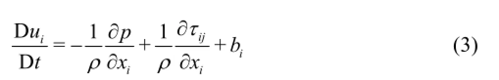
where tijis the stress tensor,biis the body force. In order to apply CIP method for advection calculation, Eq.(3) is differentiated once in terms of each direction, and the following additional governing equation is obtained.

whereRHS stands for the right hand side of Eq.(3),is the first spatial derivative. Time evaluation for Eqs.(3) and (4) is performed by a fractional step method in which time integration of those equations is divided into an advection step and two non-advection steps. The advection calculation is performed by using the CIP method, in which the following two advection equations are used.

A semi-Lagrangian scheme is used to solve Eq.(5), in which the profile of uiin each cell is approximated by a third order polynomial that is constructed by using bothuiand their first derivatives defined at the cell vertices.

The pressure is treated in a non-advection step calculation, in which the following Poisson equation is solved.

Equation (6) is assumed valid for liquid, gas and solid phase. Solution of it gives the pressure distribution in the whole computation domain. The pressure distribution obtained inside the solid body is a fictitious one, which satisfies the divergence free condition of the velocity field. The boundary condition for pressure at the interface between different phases is not necessary.

2. Interface capturing method

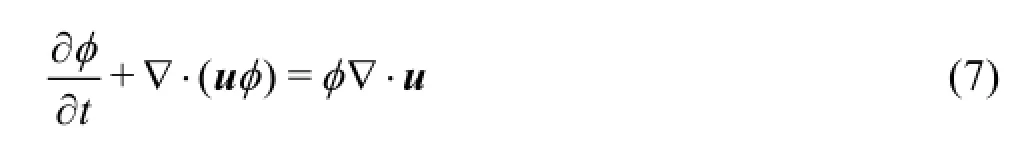
The motion of the free surface is calculated by the THINC scheme, a high-performance interfacecapturing scheme which is proposed by Xiao et al.[2]. This scheme is a kind of finite volume method which is similar to the VOF method. By using the THINC scheme, the following governing equation in a conservation form for the colour function of liquid φ(x,t)is solved.

Numerical calculation of this equation is performed by integration over a time interval [t, t+∆t]and a cellwhich gives

The fluxes in Eq.(8) are computed by a semi-Lagrangian scheme, in which a piecewise modified hyperbolic tangent function is used to approximate the profile of φinside the cell. Detailed description of the scheme can be found in Refs.[2] and [9].

3. 6-DOF motion of floating body

The floating body is considered as a rigid body in the numerical model. When the hydrodynamic forces on the body are obtained, it is not difficult to calculate translational and rotational velocities at the gravity center of the rigid body. In order to treat large amplitude ship motions such as capsizing, the rotation of the body is solved by using quaternion representation.

The fluid structure interaction is solved in an explicit way:

Step1: The motion of floating body is solved by using the hydrodynamic forces on the body which is obtained from the fluid flow simulation result.

Step 2: The fluid field is solved in which the effect of the floating body motion is treated by using the IB method.

The location of the floating body boundaries is determined by using the colour function for the solid phase φ3. We have developed a virtual particle method to calculate φ3in an easy way for 3-D cases[6], in which the body surface is defined by uniform distribution of virtual particles on it as shown in Fig.1. For a rigid body, the velocity at any particle on the body surface can be easily obtained. Then the velocity at the body boundary cell, which is required to specify as the boundary condition, can be calculated by using the velocities at surrounding particles. In the numerical procedure, the method of imposing the velocity distribution inside and on the body boundary is equivalent to adding a forcing term to the momentum equation. The following updating operation is carried out after the calculation of Eq.(3).

where u∗∗is the velocity obtained by solving Eq.(3). Such numerical treatment of the floating body is of first order accuracy. A second order immersed boundary method has also been developed by the authors and is described in the following section.

4. Improved immersed boundary method

Recently we have proposed a modified IB method[10]which is an improvement to the method proposed by Yang and Balaras[11]. There are several new contributions of our method. A simple mapping strategy for body surface tracking is newly developed which can deal with 2-D or 3-D complex surface geometry of rigid or deformable body easily. Moreover, to alleviate the pressure oscillation in the computation on a coarse grid, a new suppression scheme is introduced by dynamically alternating the weighting factor of interpolation stencils.

4.1 Body surface tracking strategy

Although the virtual particle method is easy to be extended from 2-D to 3-D, the drawback due to the use of large amount of particles is obvious. A virtual panel method is newly proposed to represent moving body surface.

In the virtual panel method, we use panels to describe the body surface. Main procedure of the method is organized as following: (1) For(M is total panel numbers), check each grid Ai( i=1, 2,…N)(Nis total grid numbers), judge which panels are possibly intersected with the grid. Then identify the cut elements. (2) During the sweeping step, judge which edges are intersected with panel, then record relevant information using binary bits by tagging corresponding bit to 1. Besides, the normal vector and the volume should be calculated in current step. (3) A ray-tracing algorithm is adopted to specify three physical phases (air, water, solid) that are occupied by one physical component through sweeping inx,y,z axial directions.

A modified IB treatment combined with level set (LS) method has been developed for moving bodies with complex geometrical boundaries. For initialization of the signed distance function, a region partition method is proposed to enhance the robustness of the sign calculation, in which a bounding box enclosed atriangle panel is used to reduce redundant calculations. To determine whether a point is inside or outside of the surface, we consider a direct method by using the surface normal vectors as shown in Fig.2(a). The sign is defined as follows:

wheren is the normal vector of the segment adjacent to pointP,A is the closest point toP. If the surface shape is a sharp corner as shown in Fig.2(a) for a 2-D case, special treatment is required. In this case, both segment normal vectors n1and n2are adjacent to vertex A. However,n1and n2cannot be used for checking relative position ofPbecause n1⋅PAand n2⋅PAhave different signs. This problem can be solved by firstly obtaining normal vector nAat the vortexA, then using the vortex normal vector to compute the sign by Eq.(10). By using an angle weighted method, the vertex normal nAis derived by the following formula.

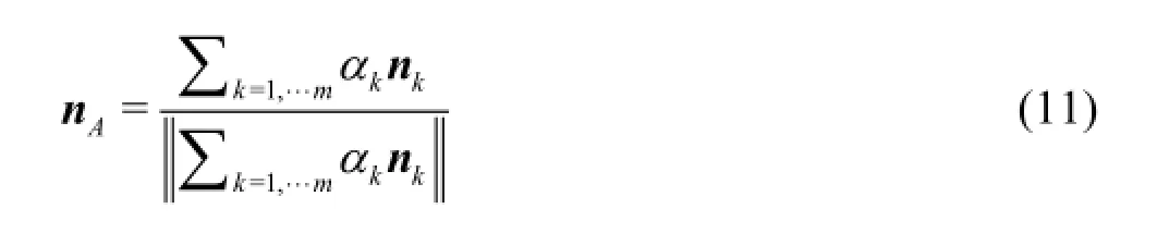
where akis the angle containing vertexA. The normal vector on the edges can be evaluated with the average of the normal vectors in two adjacent triangles.

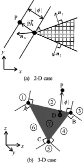
Fig.2 Method to determine a grid point Pinside or outside of the boundary

For 3-D case, the commonly used CAD stereolithography (STL) model with three vertex coordinate values is applied, in which the face normal vector are used and a region partition method is proposed to specify the sign of φP(Fig.2(b)).

For moving body cases, frequently re-initialization of the signed distance field φP( xi,t)is required. A conventional method is to perform an initialization procedure in each time step, which would be cumbersome and costly. To reduce the computation cost, a simple and efficient re-initialization method is developed by directly mapping the signed distance field from the moving reference mesh to the background mesh. For rigid body, the signed distance field is only calculated for one time, and then a mapping strategy will be used to accomplish the re-initialization procedure. In Fig.3, an example of NACA0030 foil profile is shown.

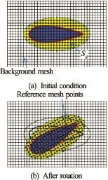
Fig.3 Mapping method for re-initialization

Fig.4 Stencils for quadratic interpolation

4.2 Interpolation scheme for velocity

In the IB method, the influence of the body is represented by adding a suitable force on the forcing points as shown by solid circles in Fig.4. The forcingpoint is the point belonging to the fluid phase with at least one neighboring solid point. The velocity vector on the forcing point is reconstructed through interpolation among the velocities at surrounding fluid grid points and the nearest body surface velocity. For a two-dimensional case, a quadratic interpolation scheme can be used as follows

Six points are required to determine the unknown coefficients, within which five stencil points belong to the fluid and one point is on the body surface, as shown in Fig.4.

5. Numerical results

Extensive validation of the CFD method described above has been carried out. In this paper, three selected examples are presented to demonstrate the performance of the method.

5.1 Numerical simulation of an anguilliform swimmer

Simulation of a 3-D flexible structure (anguilliform swimmer) in fluid with prescribed motion is presented to show the performance of the proposed improved IB method. The Reynolds number is Re = Lu/ν= 2 000, where L is the fish length,Uthe swimming velocity andνthe kinematic viscosity of water. The Strouhal number St =2 f A/ Uis defined to describe the frequency of fish tail’s swinging motion, wheref andA are the frequency and amplitude of the tail beat, respectively. The Strouhal numbers St=0.2 and 0.7 are considered for the simulation.

The kinematic form of anguilliform swimmer can be modelled by a backward traveling wave with the wave amplitude increasing almost linearly from the fish head to the tail. The following equation is often used to describe the lateral undulations of the fish.

wherex indicates the distance from the head of fish to the end,a( x)the amplitude function,ωthe angular frequency,kthe wave number of the body undulation. In this study, the following amplitude envelop a( x)is used.

In the numerical simulation,amax=0.089is used as the maximum amplitude at the fish tail.

The computational domain is a box with dimensions of6L×3L×L . A local refined stretched mesh with the mesh point number of 800×240×160 is used. A fine mesh with constant mesh spacing ∆x×∆y×∆z=0.0025Lis used in the inner domain enclosed the fish body with the size of1.2 L×0.2 L×0.1L.

Computed flow pattern and pressure distribution are shown in Fig.5. In Fig.6 the vortex structures are shown by using q-criterion. The present results are comparedwell to those obtained by other numerical method[12].

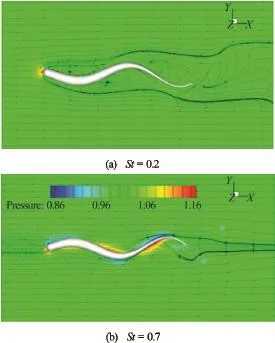
Fig.5 Pressure contours and streamlines in mid-plane of the fish

Fig.6 3-D vortex structures visualized by q-criterion for anguilliform swimmer

5.2 Prediction of added resistance in short waves

As an application to ship hydrodynamics, numerical prediction of added resistance in short waves for a container ship is carried out. Since the proposed CIP based Cartesian grid method can treat nonlinear free surface phenomena including wave reflection and breaking at the bow, this method is considered to be capable of prediction of added resistance in short waves. Numerical simulations are performed in a PC cluster system with 64 nodes. The grid point number is 640×160×200 and the computation domain is divided into 16 sub-domains for parallel computation.

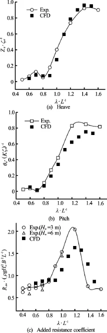
Fig.7 Comparison of RAOs between experiment and CFD

Figure 7 shows a comparison of RAOs between CFD and experiment. Good agreement is found for the heave motion. The computed pitch motion is lower than the experiment for λ/L ＞1.0. As a consequence, the predicted added resistance forλ/L ＞1.0does not compare well to the experiment. Insufficient computation domain size for long waves is considered as one of the reasons for such discrepancy. In Fig.8, computed wave patterns for λ/L=0.6and λ/L=1.2are shown. The wave-ship interaction is well simulated by the present CFD code. For the case of long wave, wave reflection at the side walls of the numerical wave tank is clearly seen. Nevertheless, the CFD prediction of added resistance in short waves is reasonably good for the present case.

Fig.8 Computed wave patterns for different wave lengths

Fig.9 A comparison between CFD and experiment for λ/L= 0.5

A comparison of free surface at the bow between the CFD simulation and the experimental photo for a short wave case (λ/L=0.5)is shown in Fig.9. Wavereflection and wave breaking are found in both the experiment and the numerical simulation. Small droplets due to wave breaking in the experimental photo cannot be reproduced by the CFD for the reason of insufficient grid resolution.

5.3 Numerical simulation of a floating platform

We use this numerical example to show that the proposed CFD method can be applied to simulation of ocean platforms. The target of the simulation is a new type offshore platform which is developed in RIAM for a R&D project on floating offshore wind turbine (FOWT) system, as shown in Fig.10(a). The system contains a catenary moored triangle semi-submersible platform on which multiple Windlens turbines and solar panels are installed. An experiment on the platform in regular waves has been carried out in the towing tank of RIAM with a 1/50 scale model to verify its hydrodynamic performance. Numerical simulation is carried out on the platform and compared with the experiment.

Fig.10 FOWT concept and comparison between CFD and experiment for the case of λ/L=1.3

In the co mp utation, a non- uniform grid with the gridnumberof400×280×230in x-,y -and zdirection is used for the numerical tank, and the minimum grid spaces are ∆x=0.00625L,∆y= 0.005625Land ∆z=0.00125L, respectively. The time step size is ∆t/ T =1/2000, whereTis the period of incident wave. The parallel version of the CFD code is used for the computation. Total 40 processors (x -axis: 10,y -axis: 4,z-axis: 1) are occupied for each case. The incident wave steepness is H/λ =1/25.

The free surface variation around the floating body is compared between the experiment and the computation as shown in Fig.10(b) and 10(c). In the figure, the experimental images are taken from the record of a high-speed digital video camera and the computed free surfaces are the iso-surfaces corresponding to φ1=0.5. The overall comparison shows reasonably good.

Fig.11 Time histories of the platform motion for the case of λ/L=0.95

Figure 11 shows time histories of the surge, heave and pitch motions for the case of λ/L=0.9. General comparison between CFD and experiment is good. Especially nonlinear features, which can be found inthe experiment, are successfully simulated by the CFD simulation.

6. Conclusions

Numerical simulation of viscous flow around an arbitrary body is conventionally performed by using a body fitted grid. Since this approach requires coordinate transformation and complex grid generation, computing moving bodies require regeneration of the mesh in every time step which usually cost large amount of CPU time. In contrast, the numerical approach proposed in this paper is a Cartesian grid method in which the grid is regular and unchanged with the time. The free surface is solved by an interface capturing scheme and the floating body is solved by an immersed boundary method.

Advantages of the Cartesian grid method are simpler programming, trivial effort in grid generation, lower storage requirements, and easier parallelization compared to the body fitted grid method. However, there are also disadvantages with this method, like the difficulty in achieving high numerical accuracy at the moving boundaries, such as the free surface and the body surface. In our Cartesian grid approach, we employ the CIP method to increase the accuracy of advection calculation around the free surface and the body surface. To increase the calculation accuracy for the moving body with complicated geometry, an efficient immersed boundary treatment is developed. In this paper we simply introduce our numerical method and describe some recent improvements of the code development. Three selected numerical results are presented to show that the proposed Cartesian grid method is promising in solving practical strongly nonlinear wave-body interaction problems.

[1] Yabe Y., Xiao F., Utsumi T. The constrained interpolation profile method for multiphase analysis [J]. Journal of Computational Physics, 2001, 169(2): 556-569.

[2] Xiao F., Ikebata A. An efficient method for capturing free boundaries in multi-fluid simulations [J]. International Journal for Numerical Methods Fluids, 2003, 42(2): 187-210.

[3] Hu C., Kashiwagi M. A CIP-based method for numerical simulations of violent free-surface flows [J]. Journal of Marine Science and Technology, 2004, 9(3): 143-157.

[4] Kishev Z. R., Hu C. and Kashiwagi M. Numerical simulation of violent sloshing by a CIP-based method [J]. Journal of Marine Science and Technology, 2006, 11(2): 111-122,.

[5] Hu C., Kashiwagi M. Two-dimensional numerical simulation and experiment on strongly nonlinear wave-body interactions [J]. Journal of Marine Science and Technology, 2009, 14(2): 200-213.

[6] Hu C., Sueyoshi M., Kashiwagi M. Numerical simulation of strongly nonlinear wave-ship interaction by CIP/cartesian grid method [J]. International Journal of Offshore and Polar Engineering, 2010, 20(2): 81-87.

[7] Zhao X., Hu C. Numerical and experimental study on a 2-D floating body under extreme wave conditions [J]. Applied Ocean Research, 2012, 35: 1-13.

[8] Liao K., Hu C. A coupled FDM-FEM method for free surface flow interaction with thin elastic plate [J]. Journal of Marine Science and Technology, 2013, 18(1): 1-11.

[9] Xiao F., Ii S., Chen C. Revisit to the THINC scheme: A simple algebraic VOF algorithm [J]. Journal of Computational Physics, 2011, 230(19): 7086-7092.

[10] Liu C., Hu C. An efficient immersed boundary treatment for complex moving object [J]. Journal of Computational Physics, 2014, 274: 654-680.

[11] Yang J., Balaras E. An embedded-boundary formulation for large-eddy simulation of turbulent flows interacting with moving boundaries [J]. Journal of Computational Physics, 2006, 215(1): 12-40.

[12] Borazjani I., Sotiropoulos F. Numerical investigation of the hydrodynamics of anguilliform swimming in the transitional and inertial flow regimes [J]. Journal of Experimental Biology, 2009, 212: 576-592.

(Received June 22, 2016, Revised September 28, 2016)

* Biography:Changhong HU, Male, Ph. D., Professor