JIN Jing-Bo， ZENG Qing-Cun， LIU Hi-Longn WU Lin

aInternational Center for Climate and Environment Sciences （ICCES）， Institute of Atmospheric Physics （IAP）， Chinese Academy of Sciences （CAS），Beijing， China；bCollege of Earth Science， University of Chinese Academy of Sciences， Beijing， China；cState Key Laboratory of Numerical Modeling for Atmospheric Sciences and Geophysical Fluid Dynamics （LASG）， Institute of Atmospheric Physics， Chinese Academy of Sciences， Beijing， China；

dState Key Laboratory of Atmospheric Boundary Layer Physics and Atmospheric Chemistry（LAPC）， Institute of Atmospheric Physics， Chinese Academy of Sciences， Beijing， China

The impacts of different surface boundary conditions for sea surface salinity on simulation in an OGCM

JIN Jiang-Boa，b， ZENG Qing-Cuna， LIU Hai-Longcand WU Lind

aInternational Center for Climate and Environment Sciences （ICCES）， Institute of Atmospheric Physics （IAP）， Chinese Academy of Sciences （CAS），Beijing， China；bCollege of Earth Science， University of Chinese Academy of Sciences， Beijing， China；cState Key Laboratory of Numerical Modeling for Atmospheric Sciences and Geophysical Fluid Dynamics （LASG）， Institute of Atmospheric Physics， Chinese Academy of Sciences， Beijing， China；

dState Key Laboratory of Atmospheric Boundary Layer Physics and Atmospheric Chemistry（LAPC）， Institute of Atmospheric Physics， Chinese Academy of Sciences， Beijing， China

An OGCM， LICOM2.0， was used to investigate the efects of diferent surface boundary conditions for sea surface salinity （SSS） on simulations of global mean salinity， SSS， and the Atlantic Meridional Overturning Circulation （AMOC）. Four numerical experiments （CTRL， Exp1， Exp2 and Exp3） were designed with the same forcing data-set， CORE.v2， and diferent surface boundary conditions for SSS. A new surface salinity boundary condition that consists of both virtual and real salt fuxes was adopted in the fourth experiment （Exp3）. Compared with the other experiments， the new salinity boundary condition prohibited a monotonous increasing or decreasing global mean salinity trend. As a result， global salinity was approximately conserved in EXP3. In the default salinity boundary condition setting in LICOM2.0， a weak restoring salinity term plays an essential role in reducing the simulated SSS bias， tending to increase the global mean salinity. However， a strong restoring salinity term under the sea ice can reduce the global mean salinity. The authors also found that adopting simulated SSS in the virtual salt fux instead of constant reference salinity improved the simulation of AMOC， whose strength became closer to that observed.

ARTICLE HISTORY

Revised 24 May 2016

Accepted 26 May 2016

Surface salinity； boundary condition； real salt fux；Atlantic Meridional Overturning Circulation；global mean salinity

盐度是海洋的一个基本状态变量，在海洋环流中起着重要的作用。少量的盐通量扰动都会改变海洋的经向翻转环流和海表温盐场。因此，本文使用了海洋环流模式LICOM2.0研究了不同盐度边界条件对全球总盐量、海表盐度和大西洋经圈翻转环流模拟的影响。结果表明：洋面上的弱恢复项对合理地模拟海表盐度起着重要的作用，且对全球总盐量起着递增的作用；在虚盐通量中使用模拟的海表盐度而非定常的参考盐度能够更合理地模拟大西洋经圈翻转环流；除此之外，含有实盐通量的盐度边界条件能够更好地维持全球总盐量的守恒。

1. Introduction

The surface boundary condition for sea surface salinity（SSS） plays an important role in realistically simulating the SSS and Atlantic Meridional Overturning Circulation（AMOC） when using OGCMs （Rahmstorf， Marotzke， and Willebrand 1996； Grifes et al. 2005， 2009）. A small perturbation of salt can modify the ocean's meridional circulation （Bryan 1986； Marotzke， Welander， and Willebrand 1988； Marotzke and Willebrand 1991； Weaver and Sarachik 1991； Weaver， Sarachik， and Marotzke 1991； Hofmann and Rahmstorf 2009） and cause a persistent climate drift（Rahmstorf， Marotzke， and Willebrand 1996）. Many previous studies have shown that both the mean state and climate variability can be more realistically captured when an OGCM adequately represents freshwater fux （Fw） forcing（e.g. Stoufer et al. 2006； Zhang and Busalacchi 2009； Zhang et al. 2012）. Therefore， a proper surface boundary condition for SSS is important for the performance of an OGCM.

The combination of salinity relaxation and virtual salt fux is widely used in most climate ocean models as the surface boundary condition for SSS. Relatively strong salinity restoration is required to stabilize the AMOC and control the sea salinity drift in OGCMs （Grifes et al. 2005）. In addition， weak salinity restoration is often used to correct the Fwat the sea surface， especially for precipitation （Grifes et al. 2005； Jin et al. 2016）. However，the salinity restoring condition has no physical basis，whereby its purpose is to prevent the modeled SSS from departing from the observed climatological distribution of surface salinity. Besides， Beron-Vera， Ochoa， and Ripa（2000） indicated that this kind of restoring condition does not guarantee the conservation of total salt in the ocean. The common technical method in ocean models is to remove the global mean restoring salt fux at each time step for the purpose of conserving the total salt. The surface salinity is often replaced by a reference salinity（often assumed to be 34.7 psu） in the virtual salt fux to formulate a better-posed problem （Roullet， Guillaume and Madec 2000）. However， this can cause signifcant biases in regions where SSS obviously difers from the reference state.

Table 1.Descriptions of the surface boundary conditions for SSS in the diferent experiments， and the statistics calculated from the diferent experiments.

New formulations of the salinity boundary condition can be adopted， which can improve upon the commonly used virtual salt fux with constant reference salinity by allowing for spatial correlations between Fwfux and SSS（Zeng and Mu 2002）. The purpose of this study is to compare the simulated results when adopting diferent surface boundary conditions for SSS， especially for SSS and the AMOC， and to identify the efects of the diferent terms in the salinity boundary condition on the OGCM. Following this introduction， Section 2 briefy introduces the model and experiments. In Section 3， we present results from four experiments， and a brief summary of our results is provided in Section 4.

2. Model and experimental design

The OGCM used in this paper is LICOM2.0 （Liu et al. 2012）. The model domain is between 78.5°S and 89.5°N， with a 1° zonal resolution. The meridional resolution is refned to 0.5° between 10°S and 10°N， and increases gradually from 0.5° to 1° between 10° and 20°. There are 30 levels in the vertical direction， with 10 m per layer in the upper 150 m. This resolution can resolve equatorial waves and capture the upper mixed layer and thermocline （Lin， Yu， and Liu 2013）. A detailed description of the model can be found in Liu et al. （2012）.

The surface salinity boundary condition （SSBC） in LICOM2.0 is a blend of the virtual salinity fux and two restoring terms. The formula is as follows: where Fw= E - P - R， in which E， P， and R are evaporation，precipitation， and river runof， respectively； S0is the reference salinity， which is assigned as a constant （34.7 psu）；WR is the weak restoring salinity condition in the open ocean， with a restoring timescale of 1 yr； and SR stands for the strong restoring term under sea ice， with a timescale of 30 days.

To test the responses of the OGCM to the diferent surface boundary conditions for SSS， four experiments were designed， called CTRL， Exp1， Exp2， and Exp3， respectively. Descriptions of the four experiments are given in Table 1. In order to reveal the uncertainty efects of WR on simulation，the WR term is not included in Exp1. Exp2 is the same as Exp1， but the simulated SSS is used instead of the reference salinity， S0. A real salt fux （μS） resulting from wind and wave breaking is added in Exp3， which is a new well-posed formulation for the SSBC and can be written as:

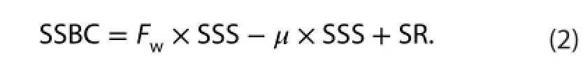
The simulated SSS is used in this formula. Here， μ is parameterized as a function of the 10-m wind speed U（μ = 0.002256U3）.

All of the external forcings used in these experiments are from CORE.v2 （Grifes et al. 2005） from Large and Yeager （2004）. Since a sea-ice model was not used in the experiments， the SSS under ice needed to be restored to the observation from WOA09 （Antonov et al. 2010）， with a restoring time scale of 30 days， in all the runs. Each experiment began from the same climatological mean salinity and temperature with a rest state. The global mean Fwfux was set to zero in every time step. All experiments were integrated for 500 years in order to reach a quasi-equilibrium deep circulation. The fnal 60 years （441—500） of the results were analyzed.

3. Results

Figure 1.Time series of global mean ocean salinity over 500 years simulated by diferent experiments.

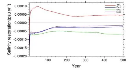
Figure 2.Time series of the surface salinity restoring term over 500 years from the diferent experiments.

Figure 1 shows the time series of global mean salinity simulated in all four experiments. There is clear distinction among the trends in global mean salinity for each experiment with a diferent SSBC. CTRL reached a quasi-equilibrium state with a gradually increasing trend of about 0.0024 psu/100 yr for the last 100 years of the integration，with its global mean salinity being 34.745 psu averaged in the last year. The SR term played a dominate role in reducing the trend in global mean salinity in the remaining experiments （Figure 2）. Since the global mean virtual salt fux （FwS0） is approximately zero， the increasing trend in global mean salinity in CTRL was mainly attributable to the efects of WR. Exp1， in which WR was excluded， exhibited a slow monotonic decreasing trend （approximately -0.0038 psu/100 yr） with a 500th-year mean salinity of 34.711 psu. Moreover， the signifcant increasing trend in Exp2 was about 0.0071 psu/100 yr during the last 100 years，which resulted from the evident positive relationship between Fwand SSS， although the decreasing efects of SR in Exp2 were also obvious （Figure 2）. The global mean salinity （34.770 psu） of the 500th year for Exp2 was the largest among the experiments. Exp3 reached a near stationary state after 100 years， with a slight negative trend of -0.0002 psu/100 yr for the last 100 years. During the last year， the value in Exp3 was 34.723 psu， which was the closest experimental result to the observed value of 34.728 psu （Table 1）. This clearly demonstrates the importance of the real salinity fux term compared with Exp2.

Comparing the results of CTRL and Exp1， it was apparent that weak SSS restoration in the open sea increased the global mean salinity， whereas strong restoration under the sea-ice region caused a decrease.

Figure 3.Simulated SSS （contours） and biases against observations from WOA09 （color shading） for （a） CTRL， （b） Exp1， （c） Exp2， and （d）Exp3.

Figure 4.Simulated annual mean meridional overturning stream-function （1 Sv = 106m3s-1） in the Atlantic for （a） CTRL， （b） Exp1， （c）Exp2， and （d） Exp3.

Figure 3 presents the biases in annual mean SSS against WOA09 （Antonov et al. 2010） for the diferent experiments. The most evident features are two large freshening SSS biases in Exp1 （Figure 3（b））: one appears between 40°S and 10°S in the Pacifc and Atlantic， and the other is located between 30°N and 45°N in the Pacifc. These large biases also occurred in Exp3 （Figure 3（d））. The root mean square diference （RMSD）was 0.686 psu in Exp3， which was closer to the CTRL value of 0.505 psu， as compared to that of Exp1 （Table 1）. The two large freshening SSS biases were mainly due to biases of the forcing feld， such as precipitation and/or RH， in CORE.v2 （Jin et al. 2016）. These large biases were partly reduced in Exp2（Figure 3（c））， especially for the subtropical western Pacifc. The reason may have been due to the biases of CORE.v2 being partly compensated by the positive relationship between Fwand SSS. Compared with CTRL， the only diference was the exclusion of the WR term in Exp1. This shows that the WR term in LICOM2.0 plays an important role in reducing the SSS bias.

However， some common biases also appeared in the four experiments. All the experiments exhibited a saltier SSS in the Laptev Sea and East Siberian Sea compared to observation， which was associated with the absence of a sea-ice component in our model. In the North Atlantic subpolar region， the SSS simulated in all of the four experiments exhibited obvious fresh biases. This was mainly because the simulated path of the Gulf Stream could not reach the North Atlantic subpolar region. As a result， there was less transportation of warm， salty water to higher latitudes. A more specifc study on this issue is needed. The corresponding SST simulated in all of the experiments was also colder in this region， as compared with WOA09 （fgure not shown）. This would have reduced the simulated evaporation fux， leading to a fresher SSS.

Figure 4 illustrates the Atlantic meridional overturning stream-function for CTRL， Exp1， Exp2， and Exp3. All of the four experiments refected the main structure of the AMOC well， indicating an upper cell between 500 m and 3，000 m and a bottom cell below. The former is related to the North Atlantic Deep Water （NADW） and the latter to the Antarctic Bottom Water.

The most striking diference between the diferent experiments was the strength of the AMOC simulated. The results from Exp2 and Exp3 （Figure 4（c） and （d）） presented the most vigorous AMOC， while CTRL （Figure 4（a）） was the weakest among the four experiments. The maximum NADW at 731 m and 36°N in CTRL was 10.8 Sv， whereas it was 11.3， 13.2， and 13.0 Sv for Exp1， Exp2， and Exp3，respectively. This strengthening is mainly related to the saltier seawater in the Labrador Sea and Norwegian Sea，but these maximum values of NADW for Exp2 and Exp3 were closer to the observed value of ～15 Sv at about 40°N（Ganachaud and Wunsch 2000， 2003； Lumpkin， Speer， and Koltermann 2008）. This indicates that the depicted AMOC strength can be improved with the virtual salt fux by adopting predicted SSS instead of the constant reference salinity. Besides， compared with Exp2， the AMOC simulated in Exp3 did not change much， since the SSS diference between Exp2 and Exp3 was minimal in the high latitudes of the North Atlantic （fgure not shown）.

4. Discussion and conclusion

This study investigated the efects of diferent surface boundary conditions for SSS on simulations of global mean salinity， SSS and the AMOC， using an OGCM （LICOM2.0）. It was found that， in the default salinity boundary condition setting in LICOM2.0， the WR term in the open sea plays an essential role in reducing the simulated SSS bias and increasing the global mean salinity， while the SR term under the sea-ice region decreases the global mean salinity. The new surface salinity boundary condition consisting of both virtual and real salt fuxes at the oceanic surface prohibited a monotonous increasing or decreasing global mean salinity trend， and basically preserved the long-term conservation of global mean salinity. Furthermore， the simulated AMOC strength was also much closer to observations， although the freshening SSS bias was large without the WR term.

A number of biases caused by ocean dynamics were also detected， such as freshening biases in the North Atlantic and subtropical regions in the Pacifc， and a weak NADW； although， both Exp2 and Exp3 ofered some improvements in this regard. The causes of these biases need further investigation.

Acknowledgements

The authors are very grateful to Dr LIN Pengfei for valuable discussions， and Mr. YU Yi for some diagnostic programs.

Disclosure statement

No potential confict of interest was reported by the authors.

Funding

This work was partially supported by the National Basic Research Program of China ［grant number 2013CB956204］； the Strategic Priority Research Program of the Chinese Academy of Sciences［grant number XDA11010403］， ［grant number XDA11010304］；the National Natural Science Foundation of China ［grant number 41305028］.

References

Antonov， J. I.， D. Seidov， T. P. Boyer， R. A. Locarnini， A. V. Mishonov，H. E. Garcia， O. K. Baranova， et al. 2010. World Ocean Atlas 2009， Volume. 2， Salinity. S. Levitus， Ed.， 184. Washington， DC: NOAA Atlas NESDIS 69， U.S. Government Printing Ofce.

Beron-Vera， F. J.， J. Ochoa， and P. Ripa. 2000. “A Note on Boundary Conditions for Salt and Freshwater Balances.” Ocean Modeling 1: 111—118.

Bryan， F. 1986.“High-latitude Salinity Efects and Interhemispheric Thermohaline Circulations.” Nature 323: 301—304.

Ganachaud， A.， and C. Wunsch. 2000. “Improved Estimates of Global Ocean Circulation， Heat Transport and Mixing from Hydrographic Data.” Nature 408: 453—457.

Ganachaud， A.， and C. Wunsch. 2003. “Large-scale Ocean Heat and Freshwater Transports during the World Ocean Circulation Experiment.” Journal of Climate 16: 696—705.

Grifes， S. M.， A. Gnanadesikan， K. W. Dixon， J. P. Dunne， R. Gerdes，M. J. Harrison， A. Rosati， et al. 2005. “Formulation of an Ocean Model for Global Climate Simulations.” Ocean Science 1: 45—79. Grifes， S. M.， A. Biastoch， C. Böning， F. Bryan， G. Danabasoglu， E. P. Chassignet， M. H. England， et al. 2009. “Coordinated Ocean-Ice Reference Experiments （COREs）.” Ocean Modelling 26: 1—46. Hofmann， M.， and S. Rahmstorf. 2009. “On the Stability of the Atlantic Meridional Overturning Circulation.” Proceedings of the National Academy of Sciences 106 （49）: 20584—20589.

Jin， J.-B.， Q.C. Zeng， H.-L. Liu， and L. Wu. 2016. “Freshening Biases in the Freshwater Flux of Coordinated Ocean-Ice Reference Experiment Data.” Atmospheric and Oceanic Science Letters 9（5）: 361—365. doi:10.1080/16742834.2016.1203244.

Large， W.， and S. Yeager. 2004. “Diurnal to Decadal Global Forcing for Ocean and Sea-Ice Models: The Data Sets and Flux Climatologies.” NCAR/TN-460+STR， 1—105.

Lin， P. F.， Y. Q. Yu， and H. L. Liu. 2013. “Long-Term Stability and Oceanic Mean State Simulated by the Coupled Model FGOALS-S2.” Advances in Atmospheric Sciences 30: 175—192.

Liu， H. L.， P. F. Lin， Y. Q. Yu， and X. H. Zhang. 2012. “The Baseline Evaluation of LASG/IAP Climate System Ocean Model （LICOM）Version 2.0.” Acta Meteorologica Sinica 26: 318—329.

Lumpkin， R.， K. Speer， and K. Koltermann. 2008. “Transport across 48°N in the Atlantic Ocean.” Journal of Physical Oceanography 38: 733—752.

Marotzke， J.， P. Welander， and J. Willebrand. 1988. “Instability and Multiple Steady States in a Meridional-Plane Model of the Thermohaline Circulation.” Tellus a 40 （2）: 162—172.

Marotzke， J.， and J. Willebrand. 1991. “Multiple Equilibria of the Global Thermohaline Circulation.” Journal of Physical Oceanography 21: 1372—1385.

Rahmstorf， S.， J. Marotzke， and J. Willebrand. 1996. “Stability of the Thermohaline Circulation.” In The Warm Water Sphere of the North Atlantic ocean， edited by W. Krauss， 129—157. Stuttgart: Borntraeger.

Roullet， Guillaume， and Gurvan Madec. 2000. “Salt Conservation，Free Surface， and Varying Levels: A New Formulation for Ocean General Circulation Models.” Journal of Geophysical Research: Oceans 105: 23927—23942.

Stouffer， R. J.， J. Yin， J. M. Gregory， K. W. Dixon， M. J. Spelman，W. Hurlin， A. J. Weaver， et al. 2006. “Investigating the Causes of the Response of the Thermohaline Circulation to past and Future Climate Changes.” Journal of Climate 19: 1365—1387.

Weaver， A. J.， and E. S. Sarachik. 1991. “The Role of Mixed Boundary Condition in Numerical Models of the Ocean's Climate.” Journal of Physical Oceanography 21: 1470—1493.

Weaver， A. J.， E. S. Sarachik， and J. Marotzke. 1991. “Freshwater Flux Forcing of Decadal and Interdecadal Oceanic Variability.”Nature 353 （31）: 836—838.

Zeng， Qing-cun， and Mu Mu. 2002. “The Design of Compact and Internally Consistent Model of Climate System Dynamics.”Chinese J. Atmos. Sci. 26 （2）: 107—113.

Zhang， R.-H.， and A. J. Busalacchi. 2009. “Freshwater Flux （FWF）-induced Oceanic Feedback in a Hybrid Coupled Model of the Tropical Pacifc.” Journal of Climate 22 （4）: 853—879.

Zhang， R.-H.， F. Zheng， J. S. Zhu， Y. H. Pei， Q. Zheng， and Z. G. Wang. 2012. “Modulation of El Niño-Southern Oscillation by Freshwater Flux and Salinity Variability in the Tropical Pacifc.”Advances in Atmospheric Sciences 29 （4）: 647—660.

表面盐度； 边界条件； 实盐通量； 大西洋经圈翻转环流； 全球平均盐度

4 May 2016

CONTACT ZENG Qing-Cun zqc@mail.iap.ac.cn

© 2016 The Author（s）. Published by Informa UK Limited， trading as Taylor & Francis Group.

This is an Open Access article distributed under the terms of the Creative Commons Attribution License （http://creativecommons.org/licenses/by/4.0/）， which permits unrestricted use， distribution， and reproduction in any medium， provided the original work is properly cited.