Ahmad Ashfaq, Lu Yanting

1. National Astronomical Observatories / Nanjing Institute of Astronomical Optics & Technology,Chinese Academy of Sciences, Nanjing 210042, P.R. China;2. Key Laboratory of Astronomical Optics & Technology, Nanjing Institute of Astronomical Optics & Technology,Chinese Academy of Sciences, Nanjing 210042, P.R. China;3. University of Chinese Academy of Sciences, Beijing 100049, P.R. China

(Received 17 April 2015; revised 21 September 2015; accepted 19 November 2015)

Removing Random-Valued Impulse Noises by a Two-Staged Nonlinear Filtering Method

Ahmad Ashfaq1,2,3, Lu Yanting1,2*

1. National Astronomical Observatories / Nanjing Institute of Astronomical Optics & Technology,Chinese Academy of Sciences, Nanjing 210042, P.R. China;2. Key Laboratory of Astronomical Optics & Technology, Nanjing Institute of Astronomical Optics & Technology,Chinese Academy of Sciences, Nanjing 210042, P.R. China;3. University of Chinese Academy of Sciences, Beijing 100049, P.R. China

(Received 17 April 2015; revised 21 September 2015; accepted 19 November 2015)

Digital images are frequently contaminated by impulse noise (IN) during acquisition and transmission.The removal of this noise from images is essential for their further processing. In this paper, a two-staged nonlinear filtering algorithm is proposed for removing random-valued impulse noise (RVIN) from digital images. Noisy pixels are identified and corrected in two cascaded stages. The statistics of two subsets of nearest neighbors are employed as the criterion for detecting noisy pixels in the first stage, while directional differences are adopted as the detector criterion in the second stage. The respective adaptive median values are taken as the replacement values for noisy pixels in each stage. The performance of the proposed method was compared with that of several existing methods. The experimental results show that the performance of the suggested algorithm is superior to those of the compared methods in terms of noise removal, edge preservation, and processing time.

image de-noising; random-valued impulse noise; nonlinear filter; noisy pixel detection; two-stage detection and correction method; cascaded stages; directional differences

0　Introduction

In image processing, noise reduction is a necessary and challenging step, which further influences the performance of subsequent analyses. Image noises are of various types, such as amplifier noise, film grain, shot noise, speckle noise, and impulse noise. During acquisition and transmission, digital images are commonly corrupted by impulse noise (IN). There are two types of INs: fixed-valued impulse noise (FVIN) and random-valued impulse noise (RVIN)[1]. In this study, we focused on removing RVIN while preserving the details and edges of the image. Let I(i, j) and I′(i, j) be the intensity values at pixel location (i, j) of the original and noisy image, respectively, n(i, j) the noise value at location (i, j), and [Imin, Imax] the dynamic range of the intensities of the original image. Then, the IN model with noise probability p using the Bernoulli uniform noise model can be given as[2]

For FVIN, a noisy pixel can take the value of either Iminor Imax[3-4], whereas for RVIN it can be any random value between Iminand Imax[5-6].

Non-linear filtering techniques, of which median filters are an example, are used frequently to remove IN. The efficiency of the standard median filter (SMF)[1]is good but it blurs the details and edges when the noise density exceeds 50%[7-8]. Several variants of SMF, such as the adaptive median filter (AMF)[3]and center-weighted median filter (CWMF)[9],were designed to overcome this problem. These methods process all the corrupt, as well as the uncorrupt pixels, which results in blurring, distortion, or elimination of the structural details.

To achieve ideal filtering, the filter should treat only the noisy pixels without affecting the noise-free pixels and therefore a noise detection procedure must be adopted before the filtering process is performed[10].Some noise removal methods using noise detectors were proposed. For example, the tri-state median filter (TSMF)[11]integrates SMF and CWMF in a noise detection framework, the recursive adaptive center-weighted median filter (ACWMF)[12]realizes the impulse detection based on the differences between the current pixel and the outputs of a CWM filter with varying weights, and the switching median filter (SwMF)[13]detects noisy pixels using the results of four convolutions obtained from one-dimensional Laplacian operators.Besides this, wavelet transform and the contourlet based edge preserving methods were also proposed. Weng et al.[14]used translation-invariant (TI) dyadic wavelet transform to suppress the noise and Wu et al.[15]applied contourlet modulus maxima technique to high frequency image portion for edge detection during noise elimination. The disadvantages of the aforementioned decision and transformation based filters are that predefined thresholds are required and possible edge pixels in corresponding regions are not specially considered during replacement, and thus, the edge and structural details remain unrecovered. Recently, Shan and Zhu[16]presented a local similarity pattern-based method. In this method, corrupt pixels are restored using the normalized weighted sum of the good pixels in their neighborhoods. However, the selection of separate weights for a smooth and an edge region renders the filtering process complex. In the method presented in Ref. [17], a low-rank matrix approximation is used to preserve the texture detail in IN corrupted images and a weighted matrix is incorporated to estimate the distribution of spatial noises. This method is designed to detect and remove non-pointwise random-valued IN, i.e., very small noise blobs, efficiently. In the last few years, fuzzy logic-based filtering techniques have been used as a substitution for the previous noise detection and reduction methods[18-21]. For example, a hybrid filtering technique[22]detects noisy pixels using the asymmetric trimmed median filter (ATMF) and restores them by using ATMF combined with a fuzzy inference system. Fuzzy filters apply human decision-making strategies to classify noisy and noise-free pixels, but at the cost of an appropriate balance between noise elimination and edge protection.

To protect the edges, Awad[23]proposed a method that finds an optimal direction to be used as a scale to judge noisy pixels. Since the direction that has the most similar pixels is considered the optimal direction, the recovery of edges having pixels between which there is a greater difference is affected. Ebenezer et al.[24]proposed a decision-based algorithm that replaces detected noisy pixels with either the median intensity value or the intensity value of a certain nearby neighbor. This method resolves the blurring effect problem, but the three sorting steps of which it is comprised lead to a decrease in filtering efficiency. Vijayaragavan et al.[25]also contributed to blurred edge restoration and proposed a two-staged algorithm that calculates directional differences in four directions. The noisy pixel is replaced with the median value of the pixels corresponding to the directions having the least differences. This method is time-efficient, but noisy pixels that are very similar to their noise-free neighbors remain undetected and thus the filtering performance is affected. Lien et al.[26]proposed a method that uses a decision-tree-based noise detector and a complex edge preserving reconstruction design. Turkmen[27]proposed a four-phase method for the reinstatement of edges. In each phase, the noisy pixel is determined by respective statistical measures and replaced by the median value of its noise-free neighbors. This method is effective in terms of noise removal and edge restoration, but increases the processing time because the image must be scanned four times.

Here we propose a two-staged filtering method that addresses the problems of edge blurring and increases processing time encountered during RVIN removal. The proposed method is an improved and hybrid version of the techniques proposed by Vijayaragavan[25]and Turkmen[27]. In our method, the detection and correction of noisy pixels at each of the two stages are accomplished differently. The performance of the proposed method is compared with that of other median-based and some recently developed methods. Our method is found to yield a significantly better performance than other baseline methods in terms of noise removal, edge preservation, and processing time.

1　Proposed Method

The proposed algorithm comprises two cascaded noise detectors instead of four independent detectors as applied in Turkmen′s method[27]. The replacement of noisy pixels is accomplished in a different manner in each stage in contrast to Turkmen′s method[27], where the same replacement mechanism is used in all phases. In stage Ⅰ, a noisy pixel is detected by examining the mean values of the absolute differences between the test pixel and two subsets of its neighbors. If the results show that the test pixel is noisy, its value is replaced by the median value of its neighboring pixels; if the pixel is found to be noise-free, its noise-free character is verified again in the second stage. In stage Ⅱ, the detection of a noisy pixel is achieved by comparing it with its neighborhood pixels in four directions. The test pixel is considered noisy when substantial differences exist between it and the pixels along more than two directions, and the median of the pixels from these directions is then used to replace the noisy pixel. Therefore, directional differences are used in noise detection instead of in the calculation of the replacement value as in Vijayaragavan′s method[25]. The unique aspects of our method are that noise detection is based on two different criterions implemented in two stages respectively, a noise-free pixel is tested twice in one scan, and two different replacement values are used. Through this two-staged method, we detect and correct the noisy pixels in two cases. The objective of the first stage is to find the noisy pixels that are significantly different from their neighbors. The second stage uses directional differences not only to capture small-difference cases missed in stage Ⅰ, but also to differentiate edge from noisy pixels, because the directional difference technique distinguishes the directions having obvious differences from those having unobvious ones. A complete description of the proposed algorithm is given in Section 1.1.

1.1Algorithm description

Consider a gray-scale noisy image I corrupted with RVIN and a sliding square test window WTof size 3×3 centered at test pixel I(i, j), given as

(1)

(2)

(3)

The first stage of the noise detection process starts

(4)

where T1and T2are the thresholds. If the value of Eq.(4) indicates that the test pixel is noisy, it is replaced by the median value of the last seven neighboring pixels. The first most similar neighbor is excluded from the calculation of the replacement value because of its probability of being noisy. The test pixel, if detected as noise-free, will be tested again in stage Ⅱ for further assurance. In stage Ⅱ, four variables denoted byΔSare defined as the absolute differences between the intensity value of the test pixel and the mean intensity values of its neighboring pixels along four major directions, i.e., horizontal, vertical, left diagonal, and right diagonal. These four variables are calculated as

(5)

From the absolute differences given in Eq.(5), a variable cnt is defined as equals the number ofΔSthat is greater than T3, and the pixel detected as cnt noise-free in stage Ⅰ is tested again

(6)

A detected noisy pixel is replaced by the median value of pixels in the directions havingΔSgreater than T3. The rationale behind this replacement mechanism is that other elements of the discarded directions are very near to the test pixel and therefore they could also be noisy, while the pixels corresponding to the directions under cnt are noise-free. Therefore, the noisy pixel is replaced by the median value of noise-free pixels. The two-staged detection and correction method is now completed and the test window is moved to process the next pixel. The entire structure of the algorithm is depicted by the flowchart given in Fig.1.

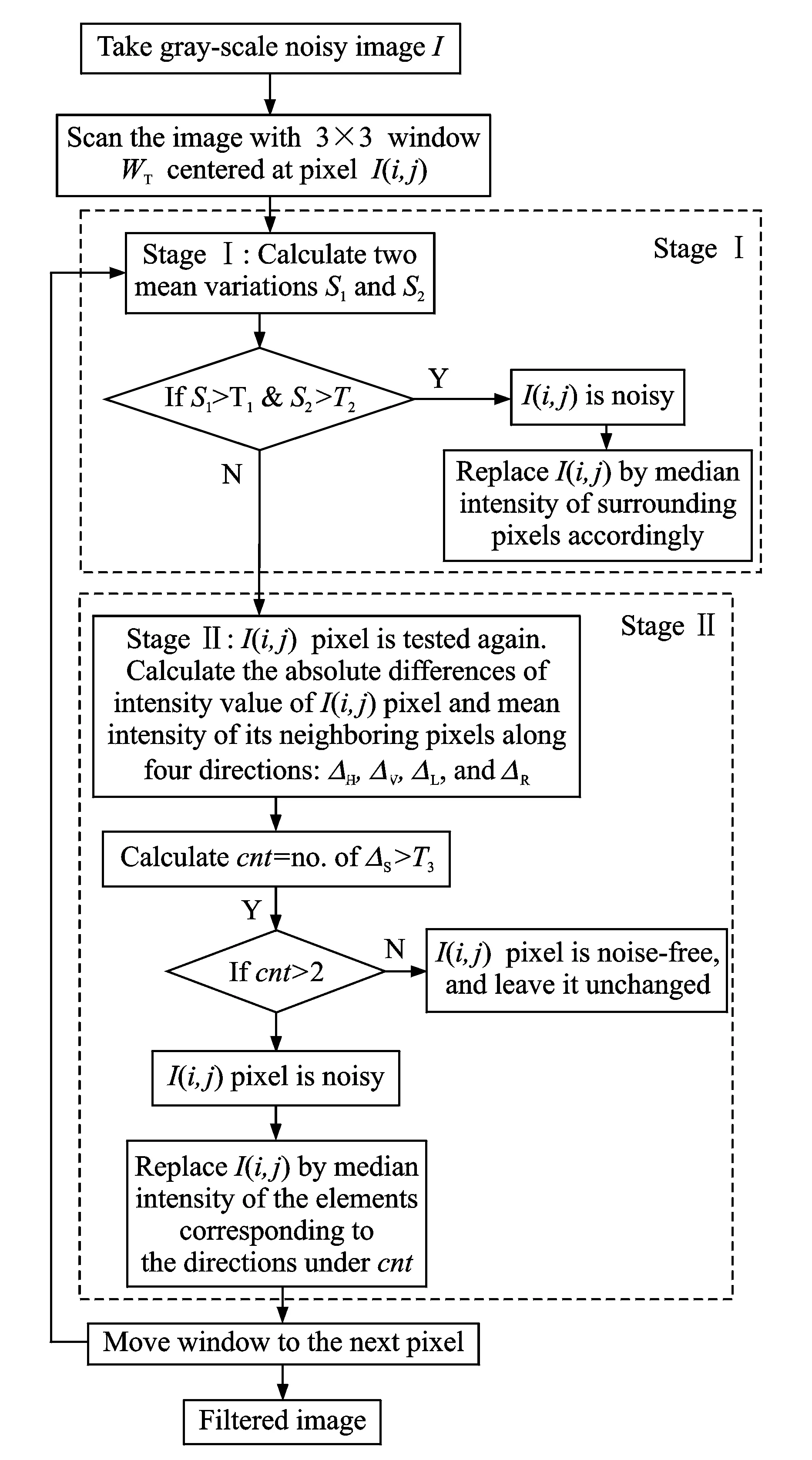
Fig.1　Flowchart of the algorithm

1.2Logic of algorithm and threshold

The logic behind using two variables in the first stage is as follows. S1helps distinguish a noisy pixel from its neighbors because the neighboring pixels of a noise-free test pixel in general possess similar characteristics. However, in the case of an image corrupted with a high noise density, the nearest three neighbors of the test pixel may also be noisy and their intensity values may be very near those of the test pixel. In this case, the mean value obtained from Eq.(2) is very small and therefore some noisy pixels remain undetected. In order to avoid corrupt pixels escaping detection, the mean of the absolute differences between the intensity values of the central pixel and the next two most similar pixels is calculated, as given in Eq.(3). The test pixel is classified as noisy if the value of Eq.(3) is larger than some threshold. In addition, if the test pixel is an edge pixel there must be at least one more pixel, having almost the same intensity, and therefore, the number of similar neighbors may exceed three. Therefore, variable S2is included to distinguish edge and noisy pixels. On the basis of the scenario stated above, the threshold values for T1and T2are kept smaller and greater, respectively. For T3, a significantly larger threshold value is selected, because in the practical scenario of stage Ⅱ not only are the corrupt pixels that have smaller differences in intensity than their neighbors detected but also edge pixels are distinguished from plane pixels. Because the test pixel varies and synchronizes its properties according to the elements in four directions, using directional differences to detect a noisy pixel in stage Ⅱ is very justifiable.

2　Experimental Results

The performance of the proposed method was tested under different noise conditions on four test images, as shown in Fig. 2. These are 8-bit gray level images and were all resized to 512 pixel×512 pixel.

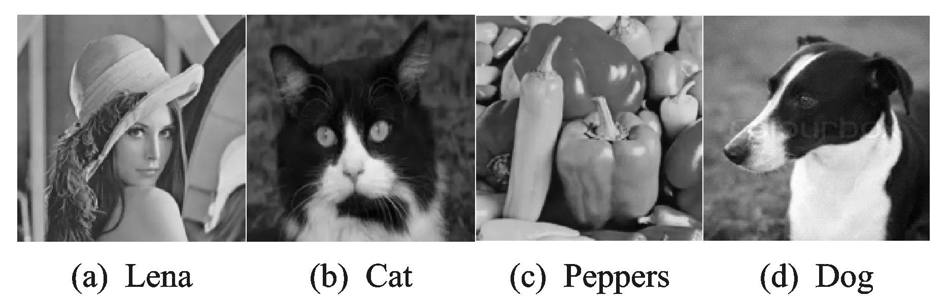
Fig.2　Test images

The filtering performance of our method was compared with those of median-based filters, including the standard median SM filter (with a 3×3 filtering window)[1], CWM filter[9], AMF[1], and the filters proposed by Ebenezer[24], where a directional difference decision-based algorithm with a 3×3 filtering window is applied, Vijayaragavan[25], where directional differences are used to calculate the replacement value with a threshold T=0.50×σ, Lien[26], which constitutes a decision-tree-based detector with thresholds of 20, 25, 40, 80, 15, and 60, and Turkmen[27], which is a four-phase method with thresholds [T1, T2, T3, T4]=[8,15,6,6]. In all the experiments, threshold values [T1, T2, T3]=[10, 16, 120] were applied in our method. The logic of calculating thresholds directly from noise observation has already been described in Section 1.2.

2.1Image restoration performance comparison

The test images used in the experiments were contaminated by RVIN with noise ratios ranging from 15% to 75%. A quantitative comparison of the restoration performances of different filters was performed using two image quality evaluation metrics: peak signal to noise ratio (PSNR) and normalized absolute error (NAE)[1,20-27]. The PSNR was calculated as

PSNR=10log10(2552/MSE)

(7)

Mean square error (MSE) was defined as

where oj, kand fj, krepresent the original and filtered images of size M×N, respectively. A larger value of PSNR reflects a higher quality of the reconstructed image. NAE was calculated as

(8)

A larger NAE value means the quality of the filtered image is poor.

All the experiments were repeated 10 times on each test image corrupted with different noise densities and then the average PSNR and NAE values of the proposed and other comparison filters were calculated, as listed in Table 1. The PSNR and NAE statistics show that SMF, AMF, CWMF, and Ebenezer′s method do not give satisfactory results as compared to the other methods. Among the remaining four methods, our method performs fairly well as compared to Turkmen′s method, and much better than Vijayaragavan′s and Lien′s methods. In Turkmen′s method, the most similar three neighbors having a chessboard distance equal to two are used as a detector that identifies the corrected pixels as noisy. Therefore, the pixels that are corrected in phase Ⅰ are changed in phase Ⅱ, resulting in low PSNR and high NAE values. In contrast, our proposed method corrects only those noisy pixels in stage Ⅱ that were missed in stage Ⅰ, and therefore, each noisy pixel is corrected in either stage Ⅰ or stage Ⅱ, but not both. Similarly, in Vijayaragavan′s method the replacement value is calculated on the basis of pixels in specific directions, and therefore, the probability that edge pixels are used in the replacement value increases. This results in blurred edges as well as poor filtering.

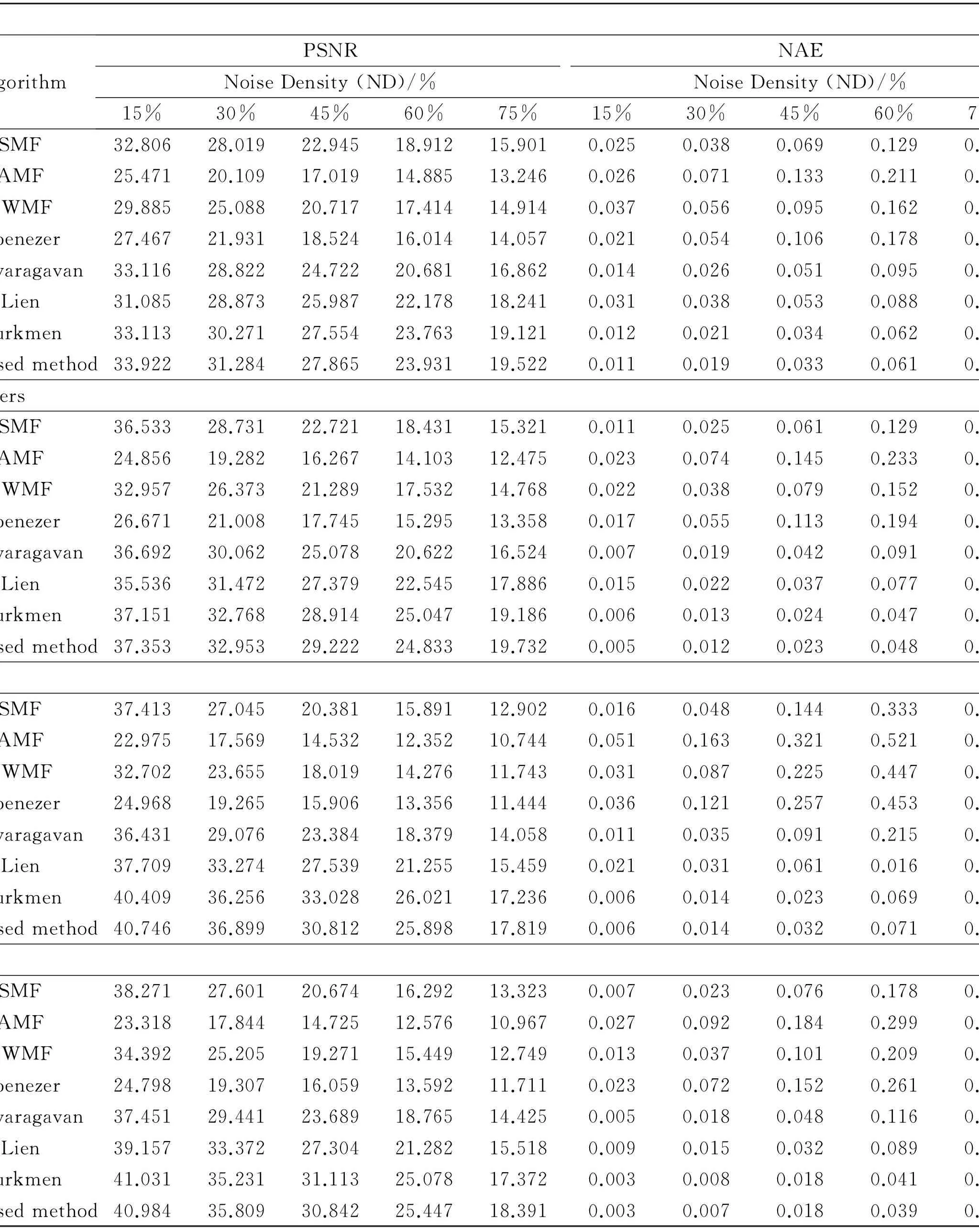
Table 1　Quantitative results on four test images corrupted with RVIN of different densities

2.2Processing time

A comparison of the processing time of the proposed and other baseline filters is given in Table 2. SMF, AMF, CWMF, and Ebenezer′s method are faster but yield worse results than the other three methods. Lien and Turkmen′s methods are slower than all the baseline methods. The reason for this is that the image is scanned four times and a variable sized window is used in Turkmen′s method, while many variables are calculated in Lien′s method. The proposed algorithm is faster than Vijayaragavan, Lien, and Turkmen′s methods because of its single scan and fixed window size design. The proposed and other comparison filters were implemented using MATLAB R2013a. All the experiments were performed on a Win7-PC with Intel(R) Core(TM) i5-3320M, CPU 2.6 GHz.

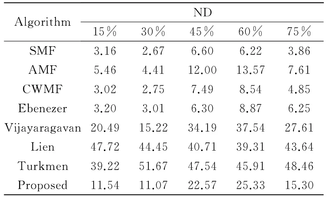
Table 2　De-noising time in seconds for Peppers image

2.3Comparison of visual performance

All the test images were corrupted with different noise densities and filtered using different methods, as shown in Figs.3, 4, respectively. The visual results show that SMF performs well in terms of filtering noises having a low density, but is not effective when applied to images having high noisy densities. The output images of AMF, CWMF, and Ebenezer′s method are very similar to each other and do not outperform SMF. However, Vijayaragavan, Lien, and Turkmen′s methods yield a significantly better visual performance. Among these three, Lien′s method preserves edges more efficiently than Turkmen′s method, which effectively filters noise. In contrast, our method shows a similar performance at first glance, but closer observation reveals that it outperforms all the other compared methods in terms of both noise removal and fine detail preservation, as shown in Fig.5. The boundary lines of the dog′s nose in Dog can be seen clearly in the image filtered by our method, whereas in those filtered by other methods the nose edges remain blurred with some corrupt blotches. Similarly, the nose and lips in Lena and the nose edges of the cat in Cat are sharper and better distinguished in the images filtered by the proposed method. Therefore, our method is efficient in terms of edge preservation. The four-phased methodology of Turkmen confuses edge and plane surface noisy pixels, and thus, pixels at sharp edges receive values similar to those of plane surface pixels, which results in blurred edges. The isolation module in Lien′s method affects the filtering performance. Similarly, when the edge pixels are used in the calculation of replacement values in Vijayaragavan′s method, the edges are expanded toward the plane surface, which renders noisy and edge pixels indistinguishable. As the intensity values of the noisy pixels are random and the number of pixels similar to a noisy pixel is changed randomly, it is appropriate to examine the noisy pixels twice, as in the proposed method. In our method, obvious noise is corrected at stage Ⅰ and missed noisy pixels are rectified at stage Ⅱ, and therefore, two different replacement values calculated by different methods are used, which enhance the proficiency of edge protection. Thus, the proposed method exhibits the best visual performance with the preservation of trivial details.

Fig.3　Noisy images with different noise ratios

2.4Selection of threshold parameters

Three threshold parameters, T1, T2, and T3,were used in our experiments. The values of parameters usually influence the results significantly. In this subsection, we describe three sets of experiments conducted to show that [T1, T2, T3]=[10,16,120] are the best parameters that can be used in image de-noising experiments. These three sets of experiments were all performed on the Lena image. In each set of experiments, the values of two parameters were fixed while the value of the remaining parameter was varied. The PSNR results of this series of experiments are plotted in a curve in Fig.6. First, we set the values of parameters T2and T3to be 16 and 120, respectively, to analyze the influence of T1on the filtering performance. It is obvious from the graph of T1that the PSNR value increases as the threshold increases until it reaches an optimum PSNR value and then decreases again with a further increase in T1. Threshold T1gives the best results in the range [8,12] and the optimum threshold is approximately 10. Second, we fixed T1and T3at values 10 and 120, respectively, to determine the effect of T2on the PSNR value. Threshold T2yields the best performance in the range [13, 20] and the maximum PSNR value is obtained at T2= 16. Third, for threshold T3our method performs well in the range [117,123], when the values of T1and T2are fixed at 10 and 16, respectively. The highest PSNR value is attained at T3= 120.

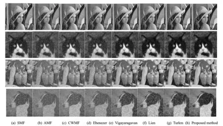
Fig.4　Visual results for restoring Lena, Cat, Peppers, and Dog corrupt images with noise ratios of 30%, 45%, 60%, and 75%, respectively

Fig.5　Edge preservation results for restoring Lena, Cat, and Dog corrupt images with noise ratios of 15%, 45%, and 75%, respectively

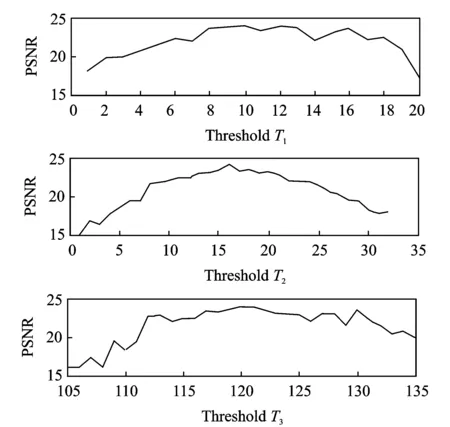
Fig.6　Dependence of PSNR on parameters T1, T2and T3 for Lena image

3　Conclusions

In this paper, a two-staged nonlinear filtering algorithm was proposed. In the first stage of our method, noisy pixels are detected using nearest neighbors, while in the second stage noisy pixels are detected using directional differences. The replacement value in stage Ⅰ is calculated using the median value of all neighboring pixels, except the first most similar one, whereas the median value of elements in specific directions is used to calculate the replacement value in stage Ⅱ. The proposed algorithm was tested on images contaminated with different noise densities. The experimental results disclose that the proposed method exhibits a better performance than other methods in terms of both noise removal and processing time. Furthermore, because of the dual check of a noisy pixel in two cascaded stages, our method outperforms all other comparison methods in terms of edge and minor detail preservation. To summarize, our method is efficient in terms of processing time, noise removal, graphic appearance, and edge preservation. Future work will focus on improving the proposed method to make it appropriate for processing the color images and removing other types of noise.

Acknowledgements

This work was supported by the Opening Project of Key Laboratory of Astronomical Optics & Technology, Nanjing Institute of Astronomical Optics & Technology, Chinese Academy of Sciences (No. CAS-KLAOT-KF201308), and partly by the special funding for Young Researcher of Nanjing Institute of Astronomical Optics & Technology, Chinese Academy of Sciences (Y-12).

[1]GONZALEZ R C, WOODS R E. Digital image processing[M]. 3rd Ed. USA: Upper Saddle River, NJ Prentice Hall, Inc., 2006: 122-126.

[2]LUO W. An efficient detail-preserving approach for removing impulse noise in images[J]. IEEE Signal Processing Letters, 2006, 13(7): 413-416.

[3]HWANG H, HADDAD R. Adaptive median filter: New algorithms and results[J]. IEEE Transactions on Image Processing, 1995, 4(4): 499-502.

[4]CHAN R H, HO C W, NIKOLOVA M. Salt and pepper noise removal by median type noise detectors and detail preserving regularization[J]. IEEE Transactions on Image Processing, 2005, 14(10): 1479-1485.

[5]CHAN R H, HU C, NIKOLOVA M. An iterative procedure for removing random-valued impulse noise[J]. IEEE Signal Processing letters, 2004, 11(12): 921-924.

[6]CHEN T, WU H R. Space variant median filters for the restoration of impulse noise corrupted images[J]. IEEE Transaction on Analog and Digital Signal Processing, 2001, 48(8): 784-789.

[7]HUANG T S, YANG G J, TANG G Y. Fast two-dimensional median filtering algorithm[J]. IEEE Transactions on Acoustics Speech and Signal Processing, 1979,27(1): 13-18.

[8]NODES T, GALLAGHER N C, JR. The output distribution of median type filters[J]. IEEE Transactions on Communications, 1984, 32(5): 532-541.

[9]KO S J, LEE Y H. Center weighted median filters and their applications to image enhancement[J]. IEEE Transactions on Circuits and Systems, 1991, 38(9): 984-993.

[10]DONG Y Q, CHAN R H, XU S F. A detection statistic for random-valued impulse noise[J]. IEEE Transactions on Image Processing, 2007, 16(4): 1112-1120.

[11]CHEN T, MA K K, CHEN L H. Tri-state median filter for image de-noising[J]. IEEE Transactions on Image Processing, 1999, 8(12): 1834-938.

[12]CHEN T, WU H R. Adaptive impulse detection using center-weighted median filters[J]. IEEE Signal Process Letters, 2001, 8(1): 1-3.

[13]ZHANG S, KARIM M A. A new impulse detector for switching median filters[J]. IEEE Signal Processing Letters, 2002, 9(11): 360-363.

[14]WENG X, WANG H, LI H, et al. Noise reduction algorithm for MRI images based on dyadic wavelet transform[J]. Transactions of Nanjing University of Aeronautics and Astronautics, 2009, 41(6): 753-756.

[15]WU Y, ZHU L, HAO Y, et al. Edge detection of river in SAR modulus maxima and improved image based on contourlet mathematical morphology[J]. Transactions of Nanjing University of Aeronautics and Astronautics, 2014, 31(5): 478-483.

[16]SHAN J, ZHU L L. A local similarity pattern for removal of random valued impulse noise[J]. Journal of Multimedia, 2014, 9(8): 1054-1059.

[17]WANG R, PAKLEPPA M, TRUCCO E. Low-rank prior in single patches for non-pointwise impulse noise removal[J]. IEEE Transactions on Image Processing, 2015, 24(5): 1485-1496.

[18]RUSSO F, RAMPONI G. A fuzzy filter for images corrupted by impulse noise[J]. IEEE Signal Processing letters, 1996, 3(6): 168-170.

[19]SCHULTE S, NACHTEGAEL M, WITTE V D, et al. A fuzzy impulse noise detection and reduction method[J]. IEEE Transactions on Image Processing, 2006, 15(5): 1153-1162.

[20]SCHULTE S, DE WITTE V, NACHTEGAEL M, et al. Fuzzy random impulse noise reduction method[J]. Fuzzy Sets and Systems, 2007, 15(8): 270-283.

[21]MELANE T, NACHTEGAEL M, KERRE E E. Random impulse noise removal from image sequences based on fuzzy logic[J]. Journal of Electronic Imaging, 2011,20(1): 13-24.

[22]PUSHPAVALLI R, SIVARAJDE G. A hybrid filtering technique for random valued impulse noise elimination on digital images[J]. ACEEE International Journal on Signal and Image Processing, 2013, 4(3): 9-16.

[23]AWAD A S. Standard deviation for obtaining the optimal direction in the removal of impulse noise[J]. IEEE Signal Processing Letters, 2011, 18(7): 407-410.

[24]SRINIVASAN K S, EBENEZER D. A new fast and efficient decision-based algorithm for removal of high-density impulse noises[J]. IEEE Signal Processing Letters, 2007, 14(3): 189-192.

[25]VIJAYARAGAVAN R, SEETHARAMAN R. Removal of random valued impulse noise by directional mean filter using statistical noise based detection[J]. International Journal of Computer Applications, 2012, 46(10): 14-18.

[26]LIEN C Y, HUANG C C, CHEN P Y, et al. An efficient denoising architecture for removal of impulse noise in images[J]. IEEE Transactions on Computers, 2013, 62(4): 631-643.

[27]TURKMEN I. A new method to remove random-valued impulse noise in images[J]. International Journal of Electronics and Communications, 2013, 67(9): 771-779.

Mr. Ahmad Ashfaq is pursuing his Ph.D. degree in computer science at Nanjing Institute of Astronomical Optics and Technology (NIAOT). His research interests include image processing, pattern recognition, interferogram analysis, and machine learning techniques suitable for assessment problems.

Dr. Lu Yanting is an engineer at NIAOT. Her research interests include pattern recognition, machine learning, and medical image processing and analysis.

(Executive Editor: Zhang Tong)

, E-mail address: ytlu@niaot.ac.cn.

How to cite this article: Ahmad Ashfaq, Lu Yanting. Removing random-valued impulse noises by a two-staged nonlinear filtering method [J]. Trans. Nanjing Univ. Aero. Astro., 2016, 33(3):329-338.

http://dx.doi.org/10.16356/j.1005-1120.2016.03.329

TP391Document code:AArticle ID:1005-1120(2016)03-0329-10