Peng LIU，Jianning SUN*，2，and Lidu SHEN

1School of Atmospheric Sciences&Institute for Climate and Global Change，Nanjing University，Nanjing210023，China

2Jiangsu Provincial Collaborative Innovation Center of Climate Change，Nanjing210023，China

Parameterization of Sheared Entrainment in a Well-Developed CBL.Part I: Evaluation of the Scheme through Large-Eddy Simulations

Peng LIU1，Jianning SUN*1，2，and Lidu SHEN1

1School of Atmospheric Sciences&Institute for Climate and Global Change，Nanjing University，Nanjing210023，China

2Jiangsu Provincial Collaborative Innovation Center of Climate Change，Nanjing210023，China

（Received 10 October 2015；revised 2 February 2016；accepted 23 May 2016）

The entrainment fl ux ratioAeand the inversion layer（IL）thickness are two key parameters in a mixed layer model.Aeis de fi ned as the ratio of the entrainment heat fl ux at the mixed layer top to the surface heat fl ux.The IL is the layer between the mixed layer and the free atmosphere.In this study，a parameterization ofAeis derived from the TKE budget in the fi rstorder model for a well-developed CBL under the condition of linearly sheared geostrophic velocity with a zero value at the surface.It is also appropriate for a CBL under the condition of geostrophic velocity remaining constant with height.LESs are conducted under the above two conditions to determine the coefficients in the parameterization scheme.Results suggest that about 43%of the shear-produced TKE in the IL is available for entrainment，while the shear-produced TKE in the mixed layer and surface layer have little e ff ect on entrainment.Based on this scheme，a new scale of convective turbulence velocity is proposed and applied to parameterize the IL thickness.The LES outputs for the CBLs under the condition of linearly sheared geostrophic velocity with a non-zero surface value are used to verify the performance of the parameterization scheme.It is found that the parameterizedAeand IL thickness agree well with the LES outputs.

large-eddy simulation，sheared convective boundary layer，entrainment fl ux ratio，inversion layer，convective velocity scale

1. Introduction

The development of the ABL over land is dominated by surface heating during the daytime.Convective activities and turbulent mixing are common within the daytime ABL，i.e.，the CBL.The top of the CBL is capped by an interface layer，where the strati fi ed free atmospheric air aloft is entrained down into the mixed layer by overshooting thermals.The entrainment process can signi fi cantly in fl uence CBL evolution and pro fi les of mean variables within the CBL（Hoxit，1974；Arya and Wyngaard，1975；Lemone et al.，1999）.It is important in NWP and air pollution models.

There have been many studies on the entrainment process.Kim et al.（2006）pointed out that much work had been done for the free CBL，whereas studies about the uncertainties in the entrainment process were quite limited compared to studies of the sheared CBL.In the past decade，research on the entrainment process has mainly focused on how to understand and parameterize the e ff ect of wind shear（Kim et al.，2003，2006；Pino et al.，2003，2006；Conzemius and Fedorovich，2006a，2006b，2007；Sun and Xu，2009）.Bulk models are often employed to describe CBL evolution.Two commonly used types of bulk models are the zeroth-order model（ZOM），which represents the inversion layer（IL）as an in fi nitesimally thin interface（Tennekes，1973），and the fi rstorder model（FOM），which assumes a certain IL thickness（Betts，1974）.The IL structure is important for CBL dynamics（Sorbjan，1996a，1996b，2004；Lewellen and Lewellen，1998；Sullivan et al.，1998；vanZanten et al.，1999；Otte and Wyngaard，2001；Kim et al.，2003，2006；Sun and Wang，2008）.Conzemius and Fedorovich（2007）reviewed previous studies of bulk models and suggested that at least the FOM is needed in order to adequately capture the entrainment process in a sheared CBL.Huang et al.（2011）demonstrated that the FOM can adequately describe not only the entrainment heat fl ux but also the entrainment fl uxes of water vapor and other conservative scalars such as carbon dioxide.

The de fi ciencies of FOMs were reviewed in Gentine et al.（2015）.In FOMs based on Betts（1974），both the potential temperature and heat fl ux pro fi les are assumed linear in the IL，and the mixed-layer top is located with the minimum heat fl ux height.Deardor ff（1979）argued that the representation of the IL in such models is oversimpli fi ed.Firstly，the ob-served maximum vertical gradient of potential temperature is generally much higher in observations than in the FOM. Secondly the minimum heat fl ux level is located above the mixed-layertop.Thirdly，theassumptionthatthemixed-layer height is equal to the minimum heat fl ux height generates a singularity for the IL growth rate equation under strong inversions.Thereafter，the IL thickness has generally been parameterized（e.g.，de fi ned as a function of the convective Richardson number）to avoid this singularity.On the other hand，the linear pro fi les are incompatible:parabolic fl ux profi les should correspond to linear pro fi les of conserved variables.Deardor ff（1979）proposed a more realistic representation of the IL—the so-called general structure model（GSM）. However，the structure of the IL in the GSM needs to be parameterized（Fedorovich and Mironov，1995；Fedorovich et al.，2004a），which limits its applicability.To overcome the limitations in previous FOMs，Gentine et al.（2015）proposed a new IL model based on a second-order polynomial for the potential temperature pro fi le，and a third-order polynomial for the heat fl ux pro fi le.This model can accurately prognosticate the growth rate of the IL，and of the mixed layer，under purely convective conditions.However，our study focuses on the entrainment process under shear conditions.It is not clear how wind shear impacts the pro fi le shapes of velocity and potential temperature and their fl uxes.In order to simplify the derivations，we use an FOM with linear pro fi les in the IL.The relative errors between the linear and curving fl ux pro fi les are discussed in this study.

The bulk model consists of a set equations for the CBL. Parameterizations of the entrainment fl ux ratio Ae（de fi ned as the ratio of entrainment heat fl ux at the top of the mixed layer to the surface heat fl ux）and IL thickness are needed for closure of the CBL equations（e.g.，Kim et al.，2006；Pino et al.，2006）.Kim et al.（2006）developed a parameterization of Aefor the CBL under the condition of height-constant geostrophic velocity（GC case）.Conzemius and Fedorovich（2007）developed a bulk CBL model under the condition of linearly sheared geostrophic velocity with a zero value at the surface（GS case），in which the Aeis not explicitly expressed and the IL thickness is parameterized assuming a constant gradient Richardson number.Note that large uncertainties exist in the parameterization of sheared entrainment.Pino et al.（2006）suggested that about 70%of TKE produced by wind shear across the IL is available for entrainment，whereas Conzemius and Fedorovich（2006a）proposed a value of 40%.Sun and Xu（2009）argued that the fraction should be 30%.Such a large discrepancy among di ff erent studies indicates that further investigation of the entrainment process is necessary for a better understanding of the CBL.

The IL thickness is another key parameter in bulk models.Pino and Vila`-Guerau De Arellano（2008）suggested that the IL thickness is a natural length scale that characterizes the shear-produced turbulence in the TKE budget at the CBL top.Kim et al.（2006）proposed three schemes to estimate the IL thickness based on di ff erent empirical considerations of the e ff ect of wind shear.Conzemius and Fedorovich（2007）developed a scheme under the assumption that the fl ux Richardson number remains at 0.25 in the entrainment zone（the layer where vertical potential temperature fl ux is negative）.However，the LES results of Pino and Vil`a-Guerau De Arellano（2008）showed the fl ux Richardson number to be larger than 0.25.Therefore，the scheme of Conzemius and Fedorovich（2007）needs further validation and the parameterization of the IL thickness should be modi fi ed.

In this paper，a parameterization scheme of Aefor a welldeveloped CBL is developed in an FOM framework.As in Conzemius and Fedorovich（2007），the CBL is assumed to develop under the condition of the GS case.The impacts of di ff erent factors on Aeare discussed.A new convective velocity scale for both buoyancy and shear e ff ects is proposed to parameterize the IL thickness.LESs are conducted to evaluate the parameterization of Aeand the performance of parameterization for the IL thickness.In a companion paper，Part II，these parameterizations are further simpli fi ed according to the characteristics of entrainment derived from the LES output，and a simple model for predicting the growth rate of the well-developed CBL is proposed and evaluated.

2. LES experiments and output

2.1. Model setup

Twenty-six CBL cases are simulated using an LES model to provide sufficient basic data in this study.The model used is DALES（the Dutch Atmospheric Large-Eddy Simulation model），which is based on the LES code of Nieuwstadt and Brost（1986）and developed by researchers from Delft University，the Royal Netherlands Meteorological Institute，Wageningen University and the Max Planck Institute for Meteorology（Heus et al.，2010）.The domain size in this study is 10.0×10.0×4.0 km3，in the x，y and z directions respectively，with grid dimensions of 256×256×400.Sullivan and Patton（2011）pointed out that the lower-order moment statistics（means，variations and fl uxes）become grid-independent when the ratio of CBL height to LES fi lter width is larger than 56.This value corresponds to their case D，in which the mesh resolution was thought to be fi ne enough to characterize the entrainment process.In the present study，the ratio of CBL height to LES fi lter width is about 31，which is slightly larger than that of case C in Sullivan and Patton（2011）.Their results showed that the lower-order moment statistics change slightly while the entrainment rate is obviously overestimated in case C.However，their sensitivity experiments indicated that the fi ner vertical resolution can improve the LES estimates of entrainment rate efficiently.Our vertical mesh resolution is closer to that in case D than case C in Sullivan and Patton（2011）.It is expected that the mesh resolution in this study will be able to describe the turbulence statistics and entrainment process reasonably.A third-order Runge—Kutta scheme with self-adaptive time stepping is used for time integration.The surface is treated as a semi-slipboundary at the bottom，and Monin—Obukhov similarity theory is applied at the lowest model level to calculate surface momentum fl ux.The top 1 km of the domain is a sponge layer and periodic boundary conditions are applied at the lateral boundaries.The closure scheme for the calculation of subgrid-scale fl uxes is based on the TKE method（Deardor ff，1980）.

For all cases in this study，the surface potential temperature fl ux is prescribed to be 0.1 K m s-1，and the potential temperature at the surface is initially set to be 300 K.The Coriolis parameterfis set to be a constant value of 10-4s-1. Halfofthecasesareconducted withalargegradientofpotential temperature［γθ=0.006 K m-1（denoted as 6）］，and the other half are conducted with a small gradient［γθ=0.003 K m-1（denoted as 3）］.Twocases are free-convectioncases（denoted as NS00），and the others are divided into two groups，i.e.，the GC and GS groups，with the geostrophic velocity along thex-direction.In the GC group，the geostrophic velocity is prescribed with three di ff erent values:10 m s-1，15 m s-1and 20 m s-1（denoted as GC10，GC15 and GC20，respectively）.In the GS group，the geostrophic velocity is zero at the surface and linearly increases with height at three different vertical gradients:10 m s-1，15 m s-1and 20 m s-1per 2 km（denoted as GS10，GS15 and GS20，respectively）.Two values of surface roughness lengths，z0=0.1 m andz0=0.01 m，are used to represent the rough surface（denoted as R）and the smooth surface（denoted as S）.The case name GC15R3 means that the simulation is conducted under the conditions of a constant geostrophic velocity of 15 m s-1，over a rough surface，withz0=0.1 m，and an initial potential temperature gradient of 3 K km-1.Results from the 26 cases are used to determine the empirical constants in the parameterization schemes.

The present study is based on linear equations of potential temperature and momentum for a horizontally homogeneous CBL.With Galilean transformation，CS cases can be easily transformed to GS cases.It is expected that the parameterizations derived from GS cases should be suitable for CS cases.However，this is not true for a nonlinear system such as the three-dimensional CBL.Furthermore，non-zero surface geostrophic velocity leads to changes in surface friction velocity and mixed-layer velocity，and consequently affects velocity and fl uxes at the CBL top.The changes in these variables are not linear.For this reason，four additional CS CBL experiments（C5S10S3，C5S15S3，C5S15S6 and C5S15R3）are conducted to validate the parameterizations derived from GS cases.The case name C5S15S3 means that the surface value of geostrophic velocity is 5 m s-1，the gradient of geostrophic velocity is 15 m s-1per 2 km，the surface is smooth（z0=0.01 m），and the gradient of potential temperature is 3 K km-1.

2.2. Pro fi les and variables in the FOM

The integration for each simulation covers 28 800 s，and the results for the period from 4800 s to 28 800 s are output at a time interval of 100 s.The horizontally averaged idealized pro fi les of potential temperature，velocity and their fl uxes can be obtained from the LES output.Figures 1 and 2 depict these LES cases and idealized pro fi les.In this paper，the mean and the fl uctuating parts of a turbulent variable are denoted with uppercase and lowercase letters；for example，Θ and θ represent the domain averaged and fl uctuating parts of potential temperature.A horizontally averaged turbulent fl ux is denoted by an overbar；for example，means horizontally averaged kinematic heat fl ux.The idealized pro fi le of Θ is assumed to vary linearly with height in all cases.Fedorovich（1995）gave the idealized pro fi le ofin the mixed layer as

wherezis height andh1is the CBL height，which is de fi ned as the height at whichfrom the LES output reaches its minimum；andare the kinematic heat fl ux at the surface and ath1respectively.Based on this equation，Aeis

Fig.1.Idealized pro fi les（solid lines）of a CBL with constant geostrophic wind（GC）.Top:horizontally averaged potential temperatureand its vertical fl uxmiddle:horizontally averagedx-component velocityUand its vertical fl ux；bottom: horizontally averagedy-component velocityVand its vertical fl uxThick dashed lines represent LES pro fi lesdash-dot lines representh0，h1andh2.The vertical axis represents height above the surface.

Fig.2.As in Fig.1，but with linearly increasing geostrophic wind（GS）.

expressed as

where h0is the fi rst zero-crossing height of thepro fi le.h2is de fi ned as the level at whichis larger than 10%of its minimumvalue，which is thesameasin Pino et al.（2006）and Conzemius and Fedorovich（2006a）.The layer from h1to h2is the so-called IL，and its thickness is Δh21=h2-h1.The layer between h0and h2is the so-called entrainment zone，and its thickness is Δh20=h2-h0.It should be noted that the de fi nition of the IL is based on the idealized pro fi le of Θ，while the entrainment zone is based on the pro fi le ofFollowing Pino et al.（2006），Θ1（the potential temperature in the mixed layer）is determined from the LES Θ pro fi le at the center of the CBL（h1/2），Θ2is determined from the LES Θ profi le towards h2，and the potential temperature jump across the IL isFollowing the approach of Fedorovich（1995），the pro fi le ofin the IL is de fi ned as a quadratic function of z if Θ linearly increases with height.Calculations show that the time-averaged relative error of the integralin the IL has a maximum value of 7.8%in GC20S6.Because the errors introduced by the linear assumption are small in all of the cases，we prefer to use the linearpro fi le in this study.Kim et al.（2006）pointed out that the linear pro fi le ofgives a larger Aethan the curving pro fi le.However，the errors of Aeare associated with the empirical constants in the parameterization scheme.They are obtained by a least squares fi t to the LES outputs.The results show that the derived Aeparameterization can perform very well（details given in section 3）.

The idealized pro fi les of the velocity components U and V are also assumed to be a linear function of z（Figs.1 and 2）.For the GC cases，U and V are constant in the mixed layer；thereby，U1and V1（velocity componets at h1）are determined from the LES velocity pro fi les at the center of the CBL（h1/2）.For the GS and CS cases，the idealized U is constant in the mixed layer，whereas the idealized V linearly increases with height in the mixed layer.Thus，the determination of U1in the GS and CS cases is the same as in the GC cases.Values of V at the surface and in the middle of the CBL（h1/2），which are denoted as Vsand V1/2，are determined from the LES pro fi le of V at 0.1h1and 0.5h1，respectively.Then，V1is given as 2V1/2-Vs.For all sheared cases，the idealized U and V are assumed to be linear functions of height in the IL.U2and V2are determined from the LES profi les of U and V towards h2.The wind jumps across the IL are ΔU=U2-U1and ΔV=V2-V1.

Looking at the idealized pro fi les of momentum fl uxes，it is found thatandbelow h1vary linearly with height in the GC cases.In the GS and CS cases，below h1is a linear function of height，whereasbelow h1is a quadratic function of z（Fedorovich，1995）.According to the idealized pro fi les，the momentum fl uxes at h1are written as

The above equations are derived by vertically integrating the momentum equations（the derivations are given in Appendix A），where Ugis geostrophic velocity；Ug，sis the surface geostrophic velocity；γuis the gradient of Ug，weis the entrainment rate，which is de fi ned as we=∂〈h1〉/∂t，〈h1〉√is the least squares fi t of h1，according to the relation h1∝to avoid a negative value of we.Fedorovich et al.（2004a）showed that h1follows this relation in the NS case.Our LES outputs show that this relation is also e ff ective in the sheared CBL cases（ fi gures presented in the companion paper，Part II）.Similarly，the departure of the idealizedandprofi les from the curving ones in the IL also introduces some errors.Calculations show that the maximum relative error ofis 8%in the sheared CBL cases.The maximum relative errors ofare 10.6%，658%and 371%in the GC，GS and CS cases，respectively.However，the LES outputs show that in the GS and CS cases，the contribution of IL wind shear to the entrainment is negligibly small in the y-direction when compared with that in the x-direction（results reported in the companion paper，Part II）.Therefore，the idealized pro fi les can characterize the IL shear e ff ect on the entrainment reasonably.

3. Parameterization of Aeand evaluation

3.1. Parameterization of Aefor sheared CBLs

The derivation begins with the TKE（E）budget in Boussinesq approximation.It is expressed as

where ρ0is the air density（Moeng and Sullivan，1994），p is the fl uctuating part of pressure，g represents the acceleration of gravity，ε is the viscous dissipation rate of TKE.The TKE storage term on the left-hand side is small compared to other terms，except in the early stage of CBL evolution（Driedonks，1982；Randall，1984）.The LES outputs indicate that after 4800s of integration，when the CBL is welldeveloped，this term is small and can be neglected.The fi rst and second terms on the right-hand side are the production rates of TKE by buoyancy and wind shear，respectively.The third term is the vertical transport rate of TKE.This is a divergence term，and thus its integration from the surface to h2should be zero（Moeng and Sullivan，1994）.ε is usually assumedtobeproportionaltoitsproductionrate（Flamantetal.，1999；Conzemius and Fedorovich，2006b；Kim et al.，2006）. Applying idealized pro fi les of potential temperature，velocity and their fl uxes，as shown in Fig.2，the vertical integration of the TKE budget can be written as（see derivation in Appendix B）

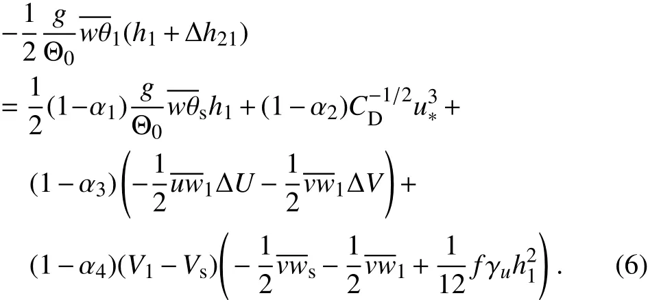
where the coefficients α1，α2，α3，and α4are the proportions of the dissipation rate to the corresponding production rate and do not vary with heightis the friction velocity，andis the surface drag coefficient.Together with the de fi nition of the convective velocity scale，i.e.，，the above equation yields the parameterization of Ae，which is expressed as

where A1=1-α1，A2=2（1-α2），A3=2（1-α3），and A4= 2（1-α4）.The terms on the right-hand side represent the contributions of the buoyancy（Term I），the surface layer shear（Term II），the IL shear（Term III）and the mixed layer shear（Term IV），respectively.Compared with the parameterization scheme for a GC case in Kim et al.（2006），the only di ff erence is that Eq.（7）has an additional term，i.e.，Term IV.If the geostrophic velocity gradient vanishes，the GS case will become a GC case（that is，Vs=V1），and Eq.（7）will turn out to be the same as the parameterization scheme for the GC case described in Kim et al.（2006）［see their Eq.（22）；the termΔU/2-ΔV/2 is equivalent to that expressed in their Eq.（5B）］.

By applying stepwise regression to outputs from all of the NS，GC and GS cases，the coefficients in Eq.（7）are given as A1=0.21，A2=0.01，A3=0.86 and A4=0.70.The value of A1is very close to the classical value of 0.2（Stull，1976；Fedorovich et al.，2004a，2004b）.From the de fi nition of A2，it can be easily shown that α2=99.5%，which means that surface shear-produced TKE dissipates locally（Conzemius and Fedorovich，2006a；Pino and Vila`-Guerau De Arellano，2008）.A3=0.86 means that the fraction of the shear-generated TKE used for the entrainment process is 43%，which is approximately the same as in Conzemius and Fedorovich（2006a）and supports the argument of Sun and Xu（2009）that the value of 1.44 for A3proposed in Pino et al.（2006）is overestimated.The stepwise regression also shows relatively large uncertainties in the determination of A4.However，the fourth term is too small to signi fi cantly infl uence the accuracy of Eq.（7）（see the results in the next section）.

In the above derivations，ε is treated as the sum of the dissipation rates of buoyancy-and shear-produced TKE.The regression of Eq.（7）to the LES outputs shows that the dissipation rate of shear-produced TKE varies in di ff erent parts of the CBL.That is，the parameterized dissipation rate εpcan be calculated as

where S is the shear production rate of TKE.Figure 3 depicts the pro fi les of εpand the forcing terms on the right-hand side of the TKE budget from the LES cases with weak inversion.εpis very close to the dissipation rate ε calculated from the LES outputs，suggesting that the coefficients in Eq.（7）are reasonable.The subgrid TKE budgets in these cases are also illustrated in Fig.3.The results indicate that the subgrid TKE is negligibly small in the IL.The cases with strong inversion have the same situation［Fig.S1 in electronic supplementary material（ESM）］.Therefore，the resolved motions dominate the TKE budget in the IL and the derived parameterizations based on the LES outputs are reasonable.Figure 4 shows that the Aeestimated by Eq.（7）agrees well with that derived from the LES outputs.As presented in previous studies，the value of Aecalculated from LES outputs fl uctuates signi fi cantly because of the fl uctuation of instantaneous LES pro fi les（calculations show that the spread of LES Aeis reduced signi fi cantly when the LES heat fl ux pro fi les are averaged over 500 s）.It is satisfactory that the value of the parameterized Aeis contained within the fl uctuations of the LES outputs.Therefore，the parameterization expressed as Eq.（7）can capture the characteristics of entrainment fl ux for a well-developed sheared CBL.

3.2. Contribution of individual terms to the parameterization scheme

Fig.3.Horizontally and 30-min averaged vertical pro fi les of the total（upper panels）and the subgrid（lower panels）TKE budget for the GC15S3，GS15S3 and C5S10S3 cases.S，B，T ε and∂E/∂t represent shear production，buoyancy production，transport and dissipation rates of TKE，respectively.εprepresents a linear combination of the shear and buoyancy production.Thin grey lines from bottom to top in each panel represent h0/h1，1 and h2/h1，respectively.

Fig.4.Entrainment heat fl ux ratios in CS cases from LES outputs（blue dots）and calculated by Eq.（7）（red dots）.

Fig.5.Each term on the right-hand side of Eq.（7）for the parameterization of Aein the GC cases.The blue dots represent Term I，the green dots represent Term II，and the red dots represent Term III.

The evolution of each term in Eq.（7）during CBL development is illustrated in Fig.5 for the GC case，and in Fig. 6 for the GS case.It is clear that Term I and Term III are the dominant terms for CBL development.The strati fi cation and wind shear have little in fl uence on Term I.Its value is about 0.18 and remains almost unchanged throughout CBL development in all of the simulation cases.Term II is alwaysvery small，albeit its value di ff ers among cases.This result suggests that Term II has little in fl uence on entrainment.The behavior of Term IIIis quitedi ff erentin the GCand GScases. Term III decreases with time and increases with strati fi cation in the GC case，whereas in the GS case it remains almost constant throughout CBL development and decreases with strati fi cation.Term IV exists in both the GS and CS cases.Figure 6 shows that this term is negligibly small in the early stage of a developing CBL.However，it increases during CBL development.Under the condition of a weak geostrophic velocity gradient，such as in GS10，Term IV can be neglected，since it remains very small throughout the entire CBL development process.On the other hand，if the geostrophic velocity gradient and h1are sufficiently large，Term IV becomes relatively large.For example，in GS20R3，at the end of the simulation，when h1is about 2000 m，the contribution of Term IV to the Aeis about 17%.However，this situation seldom happens in the real atmosphere because it is difficult for a geostrophic velocity gradient as large as that shown in case GS20R3 to occur.

In the GC case，the velocity jump across the IL increases slightly with time，but the momentum fl ux at h1decreases with time.Thus，their total shear production rate of TKE has a slight decreasing trend（Fig.S2 in ESM）.Meanwhile， the denominator of Term III）increases remarkably during this process.This is why Term III decreases with increasing CBL depth.The LES outputs indicate that a larger gradient of potential temperature can signi fi cantly enlarge the velocity jump across the IL and slightly decrease the momentum fl ux at h1（Fig.S3 in ESM）.Thereby，the shear-produced TKE and Aeenlarge under stronger strati fi cation.However，this does not mean that the growth rate of the CBL under stronger background strati fi cation increases，since the capping inversion strength also enhances，which suppresses the CBL’s development（Sun and Xu，2009）.The e ff ect of the rough surface is to enlarge the value of Term III.This is because，under such a condition，the velocity in the mixed layer is smaller and the velocity jump at the CBL top is larger，as compared to under a smooth surface condition.

In the GS case，the value of the velocity jump across the IL increases while the momentum fl uxes remain almost constant with time；thus，the shear production of TKE in the IL enhances during the CBL’s development（Fig.S4 in ESM）. Meanwhile，the denominator of Term III increases steadily during this process.Thus，the value of Term III does not change signi fi cantly.This implies that the shear production ofTKE（i.e.）isapproximately proportional toThe reduction e ff ect of strong strati fi cation on Term III means that the shear production of TKE may be proportional to the inverse of γθ.A larger geostrophic velocity gradient leads to a larger momentum fl ux at h1and velocity jump across the IL，and consequently a larger value of Term III.Figure 6 also shows that Term III is almost not in fl uenced by surface roughness.

Fig.6.As in Fig.5，but for the results in the GS cases.The cyan dots represent Term IV.Note that green dots and cyan dots overlap in some cases.

Based on the above results，it can be deduced that the shear production rate of TKE at the CBL top can be divided into two parts.One part is proportional to w3*，γuand 1/γθ；the other part is insensitive to CBL development and γθbut sensitive to surface roughness.The former part dominates in the GS case，whereas the latter works only in the GC case. In the CS case，these two parts cooperate，but the former still dominates.Thus，Term III shows a slight decreasing trend and becomes weak with larger γθ（Fig.S5 in ESM）.The expressions and meaning of these two parts are discussed in detail in the companion paper，Part II.

3.3. A new convective velocity scale

Equation（7）can be rewritten as

where wmcan be interpreted as a new characteristic convective velocity scale that includes the contributions from both the buoyancy and the wind shears in a CBL.The results in Figs.5 and 6 suggest that the characteristic convective velocity is mainly enhanced by the IL shear.In the ZOM，Eq.（10） reduces to，which agrees with the result of Tennekes（1973），Driedonks（1982），and Moeng and Sullivan（1994）that the Aecan be expressed as

For the GC case，the simpli fi ed form of Eq.（11）is often used to characterize the convective velocity scale in a sheared CBL，which includes only w*and u*on the right-hand side of the equation（Tennekes，1973；Zeman and Tennekes，1977；Tennekes and Driedonks，1981；Driedonks，1982；Boers et al.，1984；Batchvarova and Gryning，1994；Moeng and Sullivan，1994；Pino et al.，2003）.For example，Tennekes（1973） suggested that，while Moeng and Sullivan（1994）proposed thatNote that the equationonly includes the contribution of shearproduced TKE in the surface layer.Actually，it can be regarded as the simpli fi ed form of Eq.（11）by assuming thatΔV/2 is approximately proportional to［the last term of Eq.（11）is zero under the GC condition）.As mentioned in the previous section，this term is insensitive to CBL development and strati fi cation strength but sensitive to surface roughness.Our LES outputs also show that the result of Moeng and Sullivan（1994）is a good estimate of wm. However，for the GS and CS cases，the last term on the righthand side of Eq.（11）is relatively small and can be neglected（although it is not zero），but the third term on the right-hand side of Eq.（11）is closely related toIn this situation，the simpli fi ed formis not a good approximation of Eq.（11）.

4. Parameterization of the IL thickness

In the FOM，the IL thickness（Δh21=h2-h1）is a key parameter that is often used in the mixed-layer model，as described in Pino et al.（2006）and Conzemius and Fedorovich（2007）.According to parcel theory，after the overshooting thermal rises across the IL，its kinetic energy is transformed to potential energy.That is to say，Based on this assumption，Kim et al.（2006）gave the parameterization of the IL thickness in the form of

where a and b are empirical constants，and Ri is the convective Richardson number.Kim et al.（2006）proposed an empirical formula to characterize the turbulence velocity scale under the GC condition，expressed as

where c and d are empirical constants.Kim et al.（2006）provided three groups of these empirical constants.Pino et al.（2006）used this scheme in a mixed-layer model to evaluate their parameterization of Ae.By applying stepwise regression to the outputs of all the NS，GC and GS cases，cu2*in Eq.（14）is excluded（because the existence of this term makes the signi fi cance of regression reduced），and the constants are a=0.37，b=0.13 and d=0.19.When the constant b is constrained to be zero，the regression also excludes cu2*in Eq.（14），and the constants are a=2.46 and d=0.056.The exclusionofcu2*suggests that the wind shear in the surface layer has little effect on entrainment，which agrees with the result in section 3.1 that the surface shear-produced TKE dissipates locally.This scheme with di ff erent constants is denoted as KP1 and KP2，respectively（Table 1）.

In the previous section，a new convective velocity scale is proposed.We expect that it is appropriate for the estimation of IL thickness，and thus we use Eq.（12）but replace Eq.（14）with Eq.（11）.By a least squares fi t to the LES outputs of NS，GC and GS cases，the empirical constants a and b are determined to be 0.70 and 0.14，respectively.This scheme is denoted as LS1（Table 1）.

The parameterization of the IL thickness is usually evaluated by fi eld observations（e.g.，Boers et al.，1984），experiments（e.g.，Deardor ffet al.，1980）and LESs（e.g.，Fedorovich et al.，2004a）.Uncertainties in h2and Θ2determined from LES outputs will subsequently result in biases in the calculation of Δh21and ΔΘ.A positive bias of Δh21（as well as ΔΘ）causes a negative bias of Ri-1，resulting in low correlation between Δh21/h1and Ri-1（Sun et al.，2005）. For this reason，another Richardson number，RiN，which is based on the buoyancy frequencyin the free atmosphere，is used in Fedorovich et al.（2004a）.As proposedby Stull（1973），the time taken for the rising thermal to penetrate into the free atmosphere should be related to the buoyancy frequency.That isThe parameterization scheme can be written as

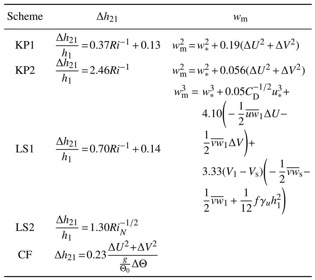
Table 1.Five di ff erent parameterization schemes of IL thickness（Δh21）.

whereaNandbNare empirical constants.For comparison purposes，we use Eq.（15）to parameterize the IL thickness and employ Eq.（11）to characterize the turbulent velocity in Eq.（16）.The least squares fi t to our LES outputs of NS，GC and GS cases yieldsaN=1.30 andbN=0.00.This scheme is denoted by LS2（Table 1）.It should be pointed out that ifEqs.（12）and（15）should be identical.The LES outputs indicate that（Fig.S6 in ESM）. The LS1 and LS2 schemes are actually equivalent；we denote them as LS1 and LS2 simply because they use di ff erent variables and have di ff erent constants.

Mahrt and Lenschow（1976）and Conzemius and Fedorovich（2006a）suggested that a balance exists between the shear production and buoyancy destruction of TKE in the entrainment zone，which can be described by the fl ux Richardson number or gradient Richardson number.Conzemius and Fedorovich（2007）set the bulk gradient Ric hardson number（Rib）in the IL to be a critical value of 0.15.The IL thickness is then given by

The constantRibis found to be 0.23 by a least squares fi t to our LES outputs of GC and GS cases.This scheme is denoted as CF（Table 1）.

In order to evaluate the performance of the above fi ve parameterization schemes for the IL thickness，the relative errors are calculated and illustrated in Fig.7.The relative error（Err）is de fi ned as

where Δh21，pis the inversion layer thickness predicted by each parameterization scheme.As mentioned above，Δh21is determined from the instantaneous LES pro fi le ofThis method can result in large errors that completely conceal di ff erences between di ff erent parameterizations.In order to reduce errors，an equal weighted nine-point moving average operator is applied to Δh21，and the result is denoted byThe CF scheme has the largest error in most cases.Further analysis shows that the bulk gradient Richardson number varies from 0.17 to 2.31 in di ff erent cases，whereas only in a few cases is the bulk gradient Richardson number very close to 0.23.This is why the CF scheme has relatively large errors in most cases.The two KP schemes apply well，although KP2 has slightly lager errors than KP1.The new empirical constants signi fi cantly improve the performance of the KP schemes（Fig.S7 in ESM），implying that the original ones proposed by Kim et al.（2006）and Pino et al.（2006）are not very representative because they were derived from only a few LES cases.LS1 is not improved in comparison with the two KP schemes；and the reason is probably that they all use the convective Richardson number（Ri），as discussed previously.However，LS2 has the best performance，and the errors are less than 20%in all cases，suggesting that theRiNscheme is more suitable for characterizing the IL thickness.

The most recent study on shear-free entrainment by means of direct numerical simulation（Garcia and Mellado，2014）suggests a two-layer model might be appropriate for studyingtheentrainmentzone.Theuppersub-layerthickness of the entrainment zone（δ）is de fi ned based on the maximum potential temperature gradient in Garcia and Mellado（2014）［see Fig.5 and Eq.（20）in their paper］.It is di ff erent to the IL thickness（Δh21）de fi ned in this study.The bottom of δ is located at the level of the maximum gradient of potential temperature that is higher than the bottom of Δh21，while the top of δ is lower than the top of Δh21.Thus，the upper sub-layer oftheentrainmentzonede fi nedinGarciaandMellado（2014）is part of the IL de fi ned in this study.Their results show that the upper sub-layer thickness（δ）of the entrainment zone is actually the mean penetration depth of an overshooting thermal，which is directly a ff ected by the background strati fi cationThe following relation is obtained［their Eq.（24）］:

Fig.7.Relative errors of the predicted capping IL thickness against the LES results.The parameterization schemes are listed in Table 1.

wherecδ=0.55 is the coefficient obtained from the direct numerical simulation results.In fact，the LS2 scheme is equivalent toFollowing the method in Garcia and Mellado（2014），δ is determined from our LES Θ profi le.The LES results show that Δh21/δ=2.44，which is quite close to 2.36，the ratio ofThis implies that the LS2 scheme is similar to Eq.（19）in a shear-free CBL，because both Δh21and δ are the overshooting distances of thermals rising in the stably strati fi ed environment.The di ff erence between the LS2 scheme and Eq.（19）is attributed to di ff erent de fi nations of Δh21and δ.Thus，in a shear-free CBL，the IL thickness is dominated by overshooting thermals.However，in a sheared CBL，the e ff ect of wind shear on the IL thickness is also important.Our results suggest that wmis suitable for characterizing the joint e ff ects of thermal overshooting and wind shear on IL thickness.

5. Conclusion and discussion

In an FOM framework，the parameterization of Aeat the top of a well-developed CBL under the GS condition is derived by vertically integrating the TKE budget.Compared to the parameterization scheme under the GC condition proposed by Kim et al.（2006）and Pino et al.（2006），our scheme includes an additional term that represents the contribution of shear-produced TKE in the mixed layer.When the geostrophic velocity gradient becomes zero，the parameterization scheme turns out to be the one under the GC condition. This scheme is also valid for the CS case.Thus，the new parameterization developed in the present study is appropriate for entrainment approximation in a well-developed CBL under di ff erent linearly sheared geostrophic velocity conditions.

The new parameterization contains four terms representing the e ff ects of the buoyancy，surface layer shear，IL shear and mixed layer shear，respectively.The buoyancy and IL shear are the dominant terms among these four terms.The LES outputs indicate that the shear-produced TKE in the surface layer dissipates locally，and 43%of the shear-produced TKE at the CBL top contributes to the entrainment，which is approximately the same as the results in Conzemius and Fedorovich（2006a）.

A new convective velocity scale in the sheared CBL is proposed.It includes the contributions of buoyancy and wind shears.In the GC cases，the convective velocity scale is equivalent to the simpli fi ed form proposed by Moeng and Sullivan（1994），in which the e ff ect of wind shear in the entire CBL can be approximately represented by the friction velocity.LES outputs show that the direct contribution of surface shear to the entrainment is relatively small.However，as pointed out by Conzemius and Fedorovich（2006a），the surface shear has an indirect e ff ect on entrainment by slowing the fl ow in the CBL interior and inducing shear at the CBL top，and it is the IL shear that enhances the entrainment.Apparently，the contribution of IL shear to the entrainment process has been considered in the simpli fi ed formula by the friction velocity.However，note that in the GS and CS cases，the simpli fi ed form of the convective velocity scale is not valid because the shear-produced TKE in the IL is mainly related to w*，the geostrophic velocity gradient and strati fi cation strength，rather than the friction velocity.

The parameterization schemes of the IL thickness proposed in previous studies are evaluated by the LES outputs. The schemes suggested by Kim et al.（2006）apply well whenthe new empirical constants are used.The empirical constants are derived by the stepwise regression to our LES outputs，which excludes the term representing the surface shear. This result supports that buoyancy and IL shear are the dominant factors of sheared entrainment.The parameterization scheme proposed by Conzemius and Fedorovich（2007）can only perform well in a few cases，because the bulk Richardson number varies widely in di ff erent cases.However，the buoyancy Richardson number approach（the RiNscheme），combined with the new convective velocity scale，can characterize the IL thickness well in all cases.

The Aeand IL thickness are important parameters in the mixed layer model.Our aim is to obtain a simpli fi ed scheme that can predict the developing process of a sheared CBL well.The parameterization scheme developed in this study represents our initial e ff orts to achieve this goal.The simplifi edmodelisfurtherexploredanddiscussedinthecompanion paper，Part II.

Finally，it is worth noting that the parameterizations proposed in this study may only be applicable for CBLs under special conditions.In the derivations we neglect the storage term in the TKE budget and only consider the linearly sheared geostrophic velocity and stable background strati fication.However，when the CBL is in its early developing stage，the storage term in the TKE budget is not negligibly small，and the entrainment process may exhibit di ff erent characteristics.There often exists a residual layer in the real atmosphere.When the CBL is growing through this layer，the entrainment process is di ff erent to that of the strati fi ed free atmosphere above the CBL.In addition，in the real atmosphere the geostrophic wind may not vary linearly with height.The applicability of the parameterization schemes under these conditions is not well investigated and needs further evaluation.These problems will be investigated in futur work.

Acknowledgements.This work was sponsored by the National Natural Science Foundation of China（Grant No.40975004）and the State Key Basic Program（973）Program（Grant No. 2013CB430100）.The numerical simulations reported in this paper were performed on the IBM Blade cluster system in the High Performance Computing Center of Nanjing University.The authors thank the anonymous reviewers，whose comments greatly helped to improve the manuscript.

Electronic supplementary material:Supplementary material is available in the online version of this article at http://dx.doi.org/ 10.1007/s00376-016-5208-x.

APPENDIX A

Derivation of

The equation of V for an idealized CBL is

By using Leibniz’s rule，the integration of Eq.（A1）across the mixed layer gives:

In IL，we assume the idealized pro fi le of V is a linear function of height and∂Δh21/∂t≈0.The integration of Eq.（A1）across the IL is

where Ug，1is the x-direction geostrophic velocity at h1.

Finally，integrating Eq.（A1）from h2to h2+ε（ε is infi nitesimal），using Leibniz’s rule and applyingto the integrated equation gives

Combining Eqs.（A2），（A3）and（A4）gives the expression offor GS and CS cases，and combining Eqs.（A2′），（A3）and（A4）gives the expression offor GC case.

APPENDIX B

Derivation of Eq.（7）

The vertical integration of the TKE budget across the CBL is

The term on the left-hand side and the third term on the right hand side are zero.Using the idealized pro fi le ofin the fi rst term on the right-hand side gives

and the second term on the right-hand side is

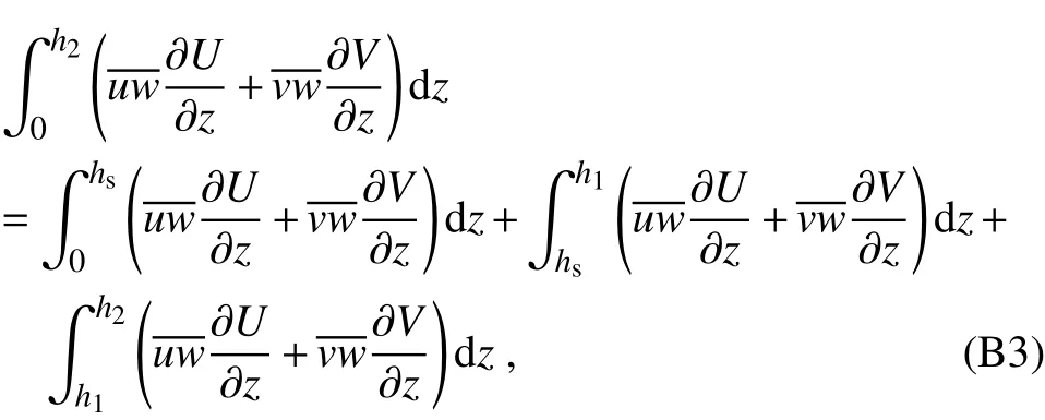
wherehsis the height of the surface layer.The same as in Kim et al.（2006），the fi rst term in Eq.（B3）is integrated such that

When the CBL is in the equilibrium state，the CBL height is sufficiently high that the surface layer depth can be neglected.By using the idealized pro fi les ofUandV，the second term in Eq.（A3）is integrated such that

Fedorovich（1995）demonstrated that the idealized pro fi le ofin the mixed layer is

Similarly，the third term in Eq.（B3）is integrated such that

The dissipation term is thought to be proportional to each production term. Therefore， the integration of Eq.（B1）is written as

REFERENCES

Arya，S.P.S.，and J.C.Wyngaard，1975:E ff ect of baroclinicity on wind pro fi les and the geostrophic drag law for the convective planetary boundary layer.J.Atmos.Sci.，32，767—778.

Batchvarova，E.，and S.-E.Gryning，1994:An applied model for the height of the daytime mixed layer and the entrainment zone.Bound.-Layer Meteor.，71，311—323.

Betts，A.K.，1974:Reply to comment on the paper“Nonprecipitating cumulus convection and its parameterization”.Quart.J.Roy.Meteor.Soc.，100，469—471.

Boers，R.，E.W.Eloranta，and R.L.Coulter，1984:Lidar observations of mixed layer dynamics:Tests of parameterized entrainment models of mixed layer growth rate.J.Climate Appl. Meteor.，23，247—266.

Conzemius，R.J.，and E.Fedorovich，2006a:Dynamics of sheared convective boundary layer entrainment.Part I:Methodological background and large-eddy simulations.J.Atmos.Sci.，63，1151—1178.

Conzemius，R.J.，and E.Fedorovich，2006b:Dynamics of sheared convective boundary layer entrainment.Part II:Evaluation of bulk model predictions of entrainment fl ux.J.Atmos.Sci.，63，1179—1199.

Conzemius，R.J.，and E.Fedorovich，2007:Bulk models of the sheared convective boundary layer:Evaluation through large eddy simulations.J.Atmos.Sci.，64，786—807.

Deardor ff，J.W.，1979:Prediction of convective mixed-layer entrainment for realistic capping inversion structure.J.Atmos. Sci.，36，424—436.

Deardor ff，J.W.，1980:Stratocumulus-capped mixed layers derivedfromathree-dimensionalmodel.Bound.-LayerMeteor.，18，495—527.

Deardor ff，J.W.，G.E.Willis，and B.H.Stockton，1980:Laboratory studies of the entrainment zone of a convectively mixed layer.J.Fluid Mech.，100，41—64.

Driedonks，A.G.M.，1982:Models andobservations ofthe growth oftheatmosphericboundarylayer.Bound.-LayerMeteor.，23，283—306.

Fedorovich，E.，1995:Modeling the atmospheric convective boundary layer within a zero-order jump approach:An extended theoretical framework.J.Appl.Meteor.，34，1916—1928.

Fedorovich，E.E.，and D.V.Mironov，1995:A model for a shearfree convective boundary layer with parameterized capping inversion structure.J.Atmos.Sci.，52，83—95.

Fedorovich，E.，R.Conzemius，and D.Mironov，2004a:Convective entrainment into a shear-free，linearly strati fi ed atmosphere:bulk models reevaluated through large eddy simulations.J.Atmos.Sci.，61，281—295.

Fedorovich，E.，and Coauthors，2004b:Entrainment into sheared convective boundary layers as predicted by di ff erent large eddy simulation codes.16th Symposium on Boundary Layers and Turbulence，Portland，ME，Amer.Meteor.Soc.

Flamant，C.，J.Pelon，B.Brashers，and R.Brown，1999:Evidence of a mixed-layer dynamics contribution to the entrainment process.Bound.-Layer Meteor.，93，47—73.

Garcia，J.R.，and J.P.Mellado，2014:The two-layer structure of the entrainment zone in the convective boundary layer.J.Atmos.Sci.，71，1935—1955.

Gentine，P.，G.Bellon，and C.C.van Heerwaarden，2015:A closer look at boundary layer inversion in large-eddy simulations and bulk models:Buoyancy-driven case.J.Atmos.Sci.，72， to be Eq.（7）.728—749.

Heus，T.，and Coauthors，2010:Formulation of the dutch atmospheric large-eddy simulation（DALES）and overview of its applications.Geoscienti fi c Model Development，3，415—444.

Hoxit，L.R.，1974:Planetary boundary layer winds in baroclinic conditions.J.Atmos.Sci.，31，1003—1020.

Huang，J.P.，X.H.Lee，and E.G.Patton，2011:Entrainment and budgets of heat，water vapor，and carbon dioxide in a convective boundary layer driven by time-varying forcing.J.Geophys.Res.，116，D06308.

Kim，S.-W.，S.-U.Park，and C.-H.Moeng，2003:Entrainment processes in the convective boundary layer with varying wind shear.Bound.-Layer Meteor.，108，221—245.

Kim，S.-W.，S.-U.Park，D.Pino，and J.V.-G.de Arellano，2006:Parameterization of entrainment in a sheared convective boundary layer using a fi rst-order jump model.Bound.-Layer Meteor.，120，455—475.

Lemone，M.A.，M.Y.Zhou，C.-H.Moeng，D.H.Lenschow，L.J. Miller，and R.L.Grossman，1999:An observational study of wind pro fi les in the baroclinic convective mixed layer.Bound.-Layer Meteor.，90，47—82.

Lewellen，D.C.，and W.S.Lewellen，1998:Large-eddy boundary layer entrainment.J.Atmos.Sci.，55，2645—2665.

Mahrt，L.，and D.H.Lenschow，1976:Growth dynamics of the convectively mixed layer.J.Atmos.Sci.，33，41—51.

Moeng，C.-H.，and P.P.Sullivan，1994:A comparison of shearand buoyancy-driven planetary boundary layer fl ows.J.Atmos.Sci.，51，999—1022.

Nieuwstadt，F.T.M.，and R.A.Brost，1986:The decay of convective turbulence.J.Atmos.Sci.，43，532—546.

Otte，M.J.，and J.C.Wyngaard，2001:Stably strati fi ed interfaciallayer turbulence from large-eddy simulation.J.Atmos.Sci.，58，3424—3442.

Pino，D.，and J.Vila`-Guerau De Arellano，2008:E ff ects of shear in the convective boundary layer:analysis of the turbulent kinetic energy budget.Acta Geophysica，56，167—193.

Pino，D.，J.Vila`-Guerau de Arellano，and P.G.Duynkerke，2003: The contribution of shear to the evolution of a convective boundary layer.J.Atmos.Sci.，60，1913—1926.

Pino，D.，J.Vila`-Guerau de Arellano，and S.-W.Kim，2006:Representing sheared convective boundary layer by zeroth-and fi rst-order-jump mixed-layer models:Large-eddy simulation veri fi cation.Journal of Applied Meteorology and Climatology，45，1224—1243.

Randall，D.A.，1984:Buoyant production and consumption of turbulence kinetic energy in cloud-topped mixed layers.J.At-mos.Sci.，41，402—413.

Sorbjan，Z.，1996a:Numerical study of penetrative and“solid lid”nonpenetrative convective boundary layers.J.Atmos.Sci.，53，101—112.

Sorbjan，Z.，1996b:E ff ects caused by varying the strength of the capping inversion based on a large eddy simulation model of the shear-free convective boundary layer.J.Atmos.Sci.，53，2015—2024.

Sorbjan，Z.，2004:Large-eddy simulations of the baroclinic mixed layer.Bound.-Layer Meteor.，112，57—80.

Stull，R.B.，1973:Inversion rise model based on penetrative convection.J.Atmos.Sci.，30，1092—1099.

Stull，R.B.，1976:The energetics of entrainment across a density interface.J.Atmos.Sci.，33，1260—1267.

Sullivan，P.P.，and E.G.Patton，2011:The e ff ect of mesh resolution on convective boundary layer statistics and structures generated by large-eddy simulation.J.Atmos.Sci.，68，2395—2415.

Sullivan，P.P.，C.-H.Moeng，B.Stevens，D.H.Lenschow，and S. D.Mayor，1998:Structure of the entrainment zone capping the convective atmospheric boundary layer.J.Atmos.Sci.，55，3042—3064.

Sun，J.N.，and Y.Wang，2008:E ff ect of the entrainment fl ux ratio on the relationship between entrainment rate and convective Richardson number.Bound.-Layer Meteor.，126，237—247.

Sun，J.N.，and Q.J.Xu，2009:Parameterization of sheared convective entrainment in the fi rst-order jump model:Evaluation through large-eddy simulation.Bound.-Layer Meteor.，132，279—288.

Sun，J.N.，W.M.Jiang，Z.Y.Chen，and R.M.Yuan，2005:A laboratory study of the turbulent velocity characteristics in the convective boundary layer.Adv.Atmos.Sci.，22，770—780，doi:10.1007/BF02918721.

Tennekes，H.，1973:A model for the dynamics of the inversion above a convective boundary layer.J.Atmos.Sci.，30，558—567.

Tennekes，H.，and A.G.M.Driedonks，1981:Basic entrainment equations for the atmospheric boundary layer.Bound.-Layer Meteor.，20，515—531.

vanZanten，M.C.，P.G.Duynkerke，and J.W.M.Cuijpers，1999: Entrainment parameterization in convective boundary layers.J.Atmos.Sci.，56，813—828.

Zeman，O.，and H.Tennekes，1977:Parameterization of the turbulent energy budget at the top of the daytime atmospheric boundary layer.J.Atmos.Sci.，34，111—123.

:Liu，P.，J.N.Sun，and L.D.Shen，2016:Parameterization of sheared entrainment in a well-developed convective boundary layer.Part I:Evaluation of the scheme through large-eddy simulations.Adv.Atmos.Sci.，33（10），1171—1184，

10.1007/s00376-016-5208-x.

*Corresponding author:Jianning SUN

Email:jnsun@nju.edu.cn